
SUFFIX ARRAYS
A Competitive Choice for Fast Lempel-Ziv Compressions
Artur J. Ferreira
1,3
, Arlindo L. Oliveira
2,4
and M´ario A. T. Figueiredo
3,4
1
Instituto Superior de Engenharia de Lisboa, Lisboa, Portugal
2
Instituto de Engenharia de Sistemas e Computadores: Investigac¸˜ao e Desenvolvimento, Lisboa, Portugal
3
Instituto de Telecomunicac¸ ˜oes, Lisboa, Portugal
4
Instituto Superior T´ecnico, Lisboa, Portugal
Keywords:
Lempel-Ziv, Lossless Data Compression, Suffix Arrays, Suffix Trees, String Matching.
Abstract:
Lossless compression algorithms of the Lempel-Ziv (LZ) family are widely used in a variety of applications.
The LZ encoder and decoder exhibit a high asymmetry, regarding time and memory requirements, with the
former being much more demanding. Several techniques have been used to speed up the encoding process;
among them is the use of suffix trees. In this paper, we explore the use of a simple data structure, named
suffix array, to hold the dictionary of the LZ encoder, and propose an algorithm to search the dictionary.
A comparison with the suffix tree based LZ encoder is carried out, showing that the compression ratios are
roughly the same. The ammount of memory required by the suffix array is fixed, being much lower than the
variable memory requirements of the suffix tree encoder, which depends on the text to encode. We conclude
that suffix arrays are a very interesting option regarding the tradeoff between time, memory, and compression
ratio, when compared with suffix trees, that make them preferable in some compression scenarios.
1 INTRODUCTION
Lossless compression algorithms of the Lempel-Ziv
(LZ) family (Salomon, 2007; Ziv and Lempel, 1977;
Storer and Szymanski, 1982) are widely used in a va-
riety of applications. These coding techniques exhibit
a high asymmetry in terms of the time and memory
requirements of the encoding and decoding processes,
with the former being much more demanding due to
the need to build, store, and search over a dictionary.
Considerable research efforts have been devoted to
speeding up LZ encoding procedures. In particular,
efficient data structures have been suggested for this
purpose; in this context, suffix trees (ST) (Gusfield,
1997; Ukkonen, 1995; McCreight, 1976; Weiner,
1973) have been proposed in (Larsson, 1996; Lars-
son, 1999).
Recently, attention has been drawn to suffix ar-
rays (SA), due to their simplicity and space efficiency.
This class of data structures has been used in such
diverse areas as search, indexing, plagiarism detec-
tion, information retrieval, biological sequence anal-
ysis, and linguistic analysis (Sadakane, 2000). In
data compression, SA have been used to encode data
with anti-dictionaries (Fiala and Holub, 2008) and
optimized for large alphabets (Sestak et al., 2008).
Linear-time SA construction algorithms have been
proposed (Karkainen et al., 2006; Zhang and Nong,
2008). The space requirement problem of the ST has
been addressed by replacing an ST-based algorithm
with another based on an enhanced SA (Abouelhoda
et al., 2004).
In this work, we show how an SA (Gusfield, 1997;
Manber and Myers, 1993) can replace an ST to hold
the dictionary in the LZ77 (also named LZ1) encod-
ing algorithm. We also compare the use of ST versus
SA, regarding time and memory requirements of the
data structures of the encoder.
The rest of the paper is organized as follows. Sec-
tion 2 describes the Lempel-Ziv 77 (Ziv and Lempel,
1977) algorithm and its variant LZSS (Storer and Szy-
manski, 1982). Sections 3 and 4 present the main fea-
tures of ST and SA, showing how to apply them to
LZ77 compression. Some implementation details are
discussed in Section 5. Experimental results are re-
ported in Section 6, while Section 7 presents some
concluding remarks.
5
J. Ferreira A., L. Oliveira A. and A. T. Figueiredo M. (2008).
SUFFIX ARRAYS - A Competitive Choice for Fast Lempel-Ziv Compressions.
In Proceedings of the International Conference on Signal Processing and Multimedia Applications, pages 5-12
DOI: 10.5220/0001935200050012
Copyright
c
SciTePress
2 LZ77 COMPRESSION
2.1 Encoding
A key feature of the Lempel-Ziv 77 (LZ77) encoding
algorithm is the use of a sliding window over the se-
quence of symbols (Salomon, 2007; Ziv and Lempel,
1977). This sliding window is composed of two sub-
windows: the dictionary and the look-ahead-buffer
(LAB). The dictionary holds the characters already
encoded, while the LAB contains the characters still
to be encoded. As a string of characters in the LAB
in encoded, the window slides to include it in the dic-
tionary (the string is said to slide in); consequently,
characters at the far end of the dictionary are dropped
by this sliding procedure (they slide out).
At each step of the LZ77 encoding algorithm, the
longest prefix of the LAB which can be found any-
where in the dictionary is determined and its position
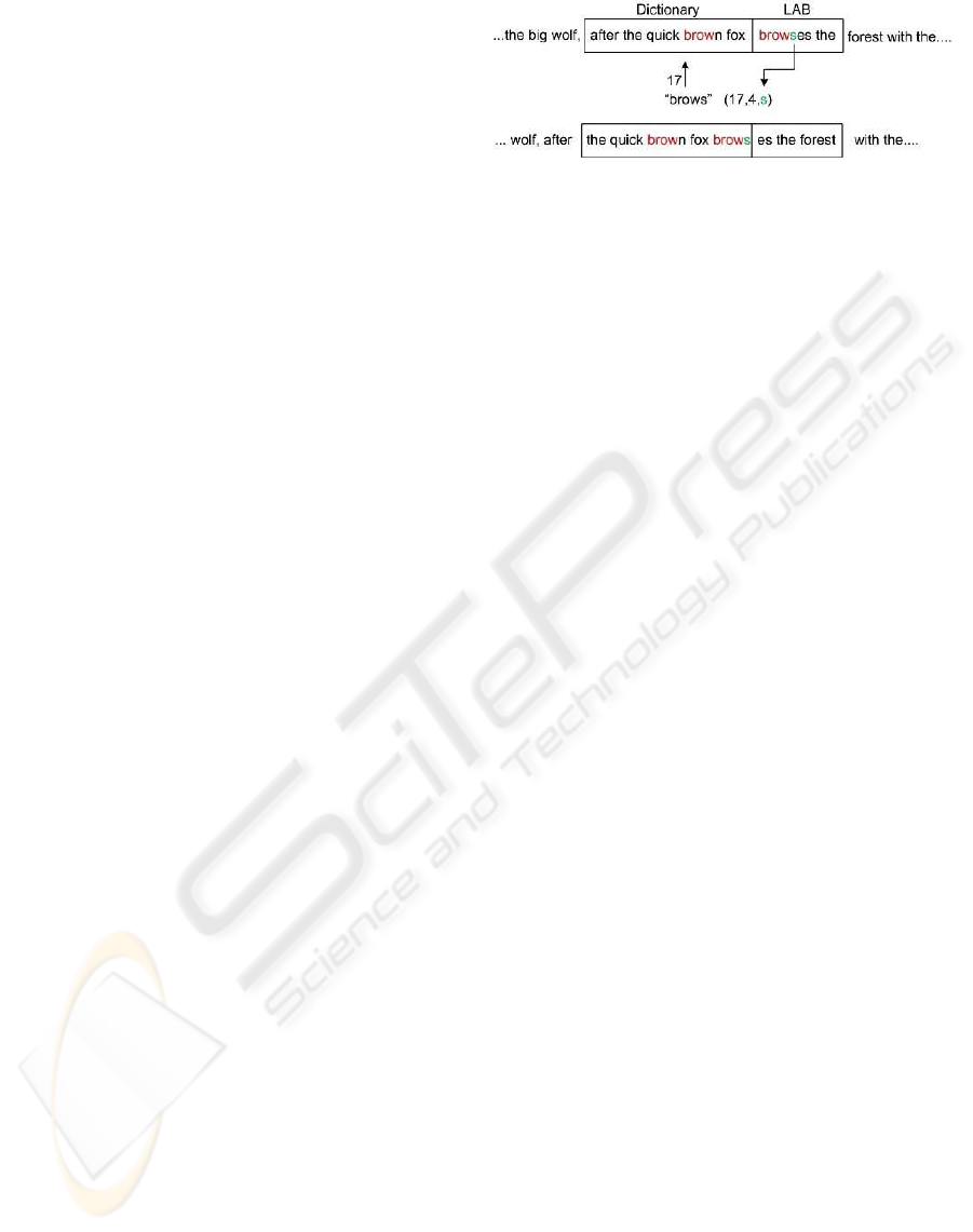
is stored. In the example of Figure 1, we find the
string of the first four symbols of the LAB (“brow”) in
position 17 in the dictionary. The encoding consists in
describing this string followed by the next symbol, by
an LZ77 token, which composed of three fields (posi-
tion, length, symbol), with the following meanings:
• position - location of the longest prefix of the
LAB found in the current dictionary; this field
uses log
2
(|dictionary|) bits, where |dictionary| is
the length of the dictionary;
• length - length of the matched substring; this re-
quires log
2
(|LAB|) bits.
• symbol - the first character, in the LAB, that does
not belong to the matched substring (the character
that breaks the match); for ASCII symbols, this
uses 8 bits.
In the example of Figure 1, the string “brows” is en-
coded by (17,4,s). Since a sequence of 5 symbols
was encoded, the window slides 5 positions forward,
thus the substring “after” performs a slide out, while
the encoded string “brows” performs a slide in. This
LZ77 token uses log
2
(|dictionary|)+log
2
(|LAB|)+8
bits, with (usually) |dictionary| ≫ |LAB|. In the ab-
sence of a match, the LZ77 token is (0,0,symbol). It’s
clear that the key component of the LZ77 encoding
algorithm is a search for the longest match between
prefixes of the LAB and the dictionary.
2.2 Decoding
The decoding process is much simpler since it in-
volves no searches. Assuming that it has been assured
that the LZ77 decoder and encoder start with the same
Figure 1: LZ77 encoding: dictionary and LAB, encoding
string “brows”, with the token (17,4,‘s’).
dictionary contents, the decoding procedure is as fol-
lows: for each LZ77 token (position,length,symbol),
the decoder
1. copies “length” symbols, starting at position “po-
sition” of the dictionary, to its output;
2. appends the symbol “symbol” to its output;
3. slides the dictionary forward so that it includes the
string just produced at its output.
Clearly, LZ77 is a very simple procedure, with very
low complexity.
2.3 LZSS Algorithm
An optimized version of LZ77, named Lempel-Ziv-
Storer-Szymanski (LZSS), was proposed in (Storer
and Szymanski, 1982). The three field token is mod-
ified to the format (bit,code); the structure of “code”
depend on value “bit” as follows:
bit = 0 ⇒ code = (character),
bit = 1 ⇒ code = (position, length).
(1)
The key idea is that, when there is a non-empty
match, there is no need to encode explicitly the fol-
lowing symbol. LZSS widely used in commercial al-
gorithms, since it typically achieves higher compres-
sion ratios than the original LZ77 algorithm. Well-
known programs such as GZIP and PKZIP are based
on LZSS. The decoding procedure for LZSS is simi-
lar to that of LZ77. Besides the modification of the
token, Storer e Szymanski (Storer and Szymanski,
1982) also proposed to keep the LAB in a circular
queue and the dictionary in a binary search tree.
3 SUFFIX TREES FOR LZ77
COMPRESSION
3.1 Suffix Trees
A suffix tree (ST) is a data structure, built from a
string, that contains the entire set of suffixes of that
string (Gusfield, 1997; Ukkonen, 1995; McCreight,
SIGMAP 2008 - International Conference on Signal Processing and Multimedia Applications
6
1976; Weiner, 1973). Given a string D of length m,
a ST consists of a direct tree with m leaves, num-
bered from 1 to m. Each internal node, except from
the root node, has two or more descendants, and each
branch corresponds to a non-empty substring of D.
The branches stemming from the same node start with
different characters. For each leaf node, i, the con-
catenation of the strings over the branches, starting
from the root to the leaf node i, yields the suffix of D
that starts at position i, that is, D[i. . . m]. Figure 2
shows the ST for string D = xabxa$, with suffixes
xabxa$
,
abxa$
,
bxa$
,
xa$
,
a$
and
$
. Each leaf node
contains the corresponding suffix number. In order
Figure 2: Suffix Tree for string D = xabxa$. Each leaf node
contains the corresponding suffix number. Each suffix is
obtained by walking down the tree, from the root node.
to be possible to build an ST from a given string, it
is necessary that no suffix of smaller length prefixes
another suffix of greater length. This condition is as-
sured by the insertion of a terminator symbol ($) at the
end of the string. The terminator is a special symbol
that does not occur previously on the string.
3.2 Encoding using Suffix Trees
An ST can be applied to obtain the LZ77/LZSS de-
scription of a string, as we describe in Algorithm 1
(Gusfield, 1997).
Algorithm 1: ST-Based LZ77 Encoding.
Inputs: D, dictionary with length |D| = m.
S, string to encode, with length |S| = n.
Output: LZ77 description of S on D.
1. Build, in O (m) time, an ST for string D;
2. Number each internal node v with c
v
, the smallest
number of all the suffixes in v’s subtree; this way,
c
v
is the left-most position in D of any copy of the
substring on the path from the root to node v;
3. To obtain the description (position, length) for the
substring S[i. . . n], with 0 ≤ i ≤ n:
a) Follow the only path from the root that matches
the prefix S[i. . . n];
b) The traversal stops at point p (not necessarily
a node), when a character breaks the match; let
depth(p) be the length of the string from the
root to p and v the first node at or below p;
c) Do position ← c
v
and length ← depth(p);
d) Output token (position, length, S[ j]), with j =
i+ length;
e) Do i ← j+ 1; if i = n stop; else goto 3.
The search in step 3b) of the algorithm obtains the
longest prefix of S[i. . . n] that also occurs in D. Fig-
ure 3 shows the use of this algorithm for the dictio-
nary D = abbacbba$; every leaf node has the number
of the corresponding suffix while the internal nodes
contain the corresponding c
v
value. In a similar man-
ner, the algorithm can be applied for LZSS compres-
sion, by modifing step 3d) in order to define the token,
according to (1). Regarding Figure 3, suppose that we
want to encode the string S = bbad; we traverse the
tree from the root to point p (with depth 3) and the
closest node at or below p has c
v
= 2, so the token
has position=2 and length=3. The token for S on D is
(2,3,‘d’).
4 SUFFIX ARRAYS FOR LZ77
COMPRESSION
4.1 Suffix Arrays
A suffix array (SA) is the lexicographically sorted ar-
ray of the suffixes of a string, holding the same infor-
mation as the ST, in an implicit way (Gusfield, 1997;
Manber and Myers, 1993). SA is an alternative to
the use of ST, in the sense that it requires (much)
Figure 3: Use of a Suffix Tree for LZ77 encoding, with dic-
tionary D = abbacbba$. Each leaf node contains the corre-
sponding suffix number, while the internal nodes keep the
smallest suffix number on their subtree (c
v
). Point p shows
the end of the path that we follow, to encode the string
S = bbad.
SUFFIX ARRAYS - A Competitive Choice for Fast Lempel-Ziv Compressions
7
less memory and has the following features (Gusfield,
1997):
• an SA uses (typically 3 ∼ 5 times) less memory
than an ST for the same string;
• an SA can be used to solve the substring problem
almost as efficiently as an ST;
• the use of an SA is more appropriate when the
alphabet of the string has high dimension.
It is possible to convert an ST into an SA in linear
time (Gusfield, 1997). An SA can also be built using a
sorting algorithm, such as “quicksort” and can be ap-
plied to obtain every occurrence of a substring within
a given string. Searching for every occurrence of a
substring consists of finding every suffix that starts
with the same character as the substring.
Let us consider the string D of length m (with m
suffixes). An SA P is a list of integers from 1 to m,
according to the lexicographic order of the suffixes of
S. For D = mississippi (with m = 11), the suffixes are
1.
mississippi
2.
ississippi
3.
ssissippi
4.
sissippi
5.
issippi
6.
ssippi
7.
sippi
8.
ippi
9.
ppi
10.
pi
11.
i
After lexicographic sorting, the result is
11.
i
8.
ippi
5.
issippi
2.
ississippi
1.
mississippi
10.
pi
9.
ppi
7.
sippi
4.
sissippi
6.
ssippi
3.
ssissippi
Thus, the SA that represents D is P =
{11, 8, 5, 2, 1, 10, 9, 7, 4, 6, 3}. Each of these in-
tegers is the suffix number and corresponds to its
position in D. Finding a substring of D can be
done by searching vector P; for instance, the set of
substrings of D that start with character i, can be
found at positions 11, 8, 5 and 2. This way, for LZ77
and LZSS encoding, we can find every substring that
starts with a given character.
The lexicographic order of the suffixes implies
that suffixesthat start with the same character are con-
secutive on SA P. This means that a binary search on
P can be used to find all these suffixes. This search
takes O (nlog(m)) time, with n being the length of the
substring to find, while m is the length of the dic-
tionary. To avoid some redundant comparisons on
this binary search, the use of longest common pre-
fix (LCP) of the suffixes, lowers the search time to
O (n+ log(m)) (Gusfield, 1997). The computation of
LCP takes O (m) time.
4.2 Encoding using Suffix Arrays
In order to perform LZ77 encoding with SA, we pro-
ceed as stated in Algorithm 2.
Algorithm 2: SA-Based LZ77 Encoding.
Inputs: D, dictionary with length |D| = m.
S, string to encode, with length |S| = n.
Output: LZ77 description of S on D.
1. Build, in O (mlog(m)) time, the SA for string D
and name it P;
2. To obtain the description (position,length) for
substring S[i. . . n], 0 ≤ i ≤ n, proceed as follows.
a) Do a binary search on vector P until we find:
i) the first position left, in which the first char-
acter of the corresponding suffix matches S[i],
that is, D[P[le ft]] = S[i];
ii) the last position right, in which the first char-
acter of the corresponding suffix matches S[i],
that is, D[P[right]] = S[i];
If no suffix starts with S[i] output (0, 0, S[i]), set
i ← i+ 1 and goto 2.
b) From the set of suffixes between P[left] and
P[right], choose the k
th
suffix, left ≤ k ≤ right,
with a given criteria (see below) obtaining a
given match; let p be the length of that match.
c) Do position ← k and length ← p.
d) Output token (position, length, S[ j]), with j =
i+ length.
e) Do i ← j+ 1; if i = n stop; else goto 2.
In step 2b), it is possible to choose among several
suffixes, according to a given criterion. If we seek
a fast search, we can choose one of the immediate
suffixes, given by left or right. If we want better com-
pression ratio, at the expense of a not so fast search,
we should choose the suffix with the longest match
with substring S[i. . . n]. LZSS encoding can be done
in a similar way, by changing step 2d) according to
the format of the token (1).
Figure 4 ilustrates LZ77 encoding with SA using
dictionary D = mississippi. We present two encoding
situations; the first a) considers S = issia, which is
SIGMAP 2008 - International Conference on Signal Processing and Multimedia Applications
8
Figure 4: LZ77/SS encoding with SA, with dictionary D =
mississippi, showing left and right indexes. In part a) we
encode S = issia, while in part b) we encode S = psi.
encoded by (5, 4, a) or (2, 4, a), depending on how we
perform the binary search and the choice of the match
(steps 3a) and 3b)); in the second example named b),
the string S = psi is encoded by (10, 1, s) or (9, 1, s)
followed by (0, 0, i). It is important to notice that SA
do not have the limitation of ST, presented in subsec-
tion 3.1: no suffix of smaller length prefixes another
suffix of greater length.
5 IMPLEMENTATION DETAILS
5.1 Suffix Trees
We have considered the ST construction algo-
rithm available at
marknelson.us/1996/08/01/
suffix-trees/
; when compared to others, this is
the code with the smallest memory requirement for
the ST data structures. This implementation (written
in C++) builds a tree from a string using Ukkonen’s
algorithm (Gusfield, 1997; Ukkonen, 1995) and has
the following main features: it holds a single version
of the string; the tree is composed of branches and
nodes; uses a hash table to store the branches and an
array for the nodes; the Hash is computed as a func-
tion of the number of the node and the first character
of the string on that branch, as depicted in Figure 5.
Two main changes in this source code were made: the
Node
was equipped with the number of its parent and
with the counter c
v
; using the number of its parent,
the code for the propagation of the c
v
values from a
node was written. After these changes, we wrote the
algorithm presented in subsection 3.2.
5.2 Suffix Arrays
We have used the SA package available at
www.cs.
dartmouth.edu/
˜
doug/sarray/
. It includes the
following functions (among others):
int sarray(int *a, int m);
int *lcp(const int *a, const char *s, int m);
Figure 5: Ilustration of ST data structures. The branch be-
tween nodes 2 and 3, with string “xay” that starts and ends
at positions 4 and 6, respectivelly. The node only contains
its suffix link.
The SA computation by
sarray
is done in time
O (mlog(m)), while the LCP computation by
lcp
takes O (m) time. Using these functions, we imple-
mented the algorithm described in Subsection 4.2.
5.3 Other Details
For both encoders (with ST and SA), we copy the con-
tents of the LAB to the end of the dictionary, only
when the entire contents of the LAB is encoded. An-
other important issue is the fact that for ST (but not
for the SA), we add a terminator symbol to end of the
dictionary, to assure that we have a valid ST. This jus-
tifies the small differences in the compression ratios
attained by the ST and SA encoders.
6 EXPERIMENTAL RESULTS
This section presents the experimental results, using
the LZ77 and LZSS encoders, for dictionaries and
LAB of different sizes. The evaluation was carried
out using standard test files from the well-known Cal-
gary Corpus
1
and Canterbury Corpus
2
. The 18 se-
lected files are listed in Table 1.
The compression tests were carried out on a ma-
chine with 2GB RAM and an Intel processor Core2
Duo CPU T7300 @ 2GHz. We measured the fol-
lowing parameters: encoding time (seconds), mem-
ory used by the encoder data structures (bytes) and
compression ratio given by
CR = 100
1−
Encoded Size
Original Size
[%], (2)
for the LZSS encoder. The memory indicator refers to
the average ammount of memory needed for every ST
1
links.uwaterloo.ca/calgary.corpus.html
2
corpus.canterbury.ac.nz/
SUFFIX ARRAYS - A Competitive Choice for Fast Lempel-Ziv Compressions
9
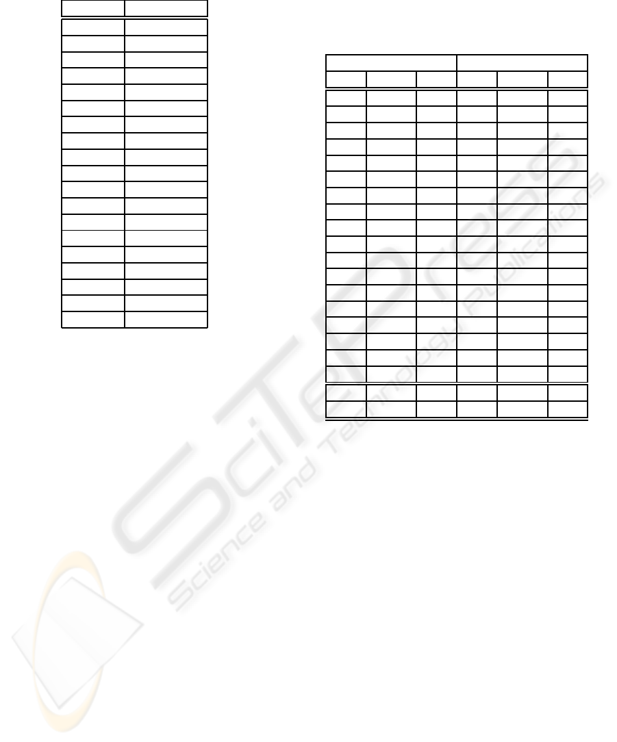
Table 1: Description of the test files selected from Calgary
Corpus and Canterbury Corpus.
File Size (bytes)
bib 111261
book1 768771
book2 610856
news 377109
paper1 53161
paper2 82199
paper3 46526
paper4 13286
paper5 11954
paper6 38105
progc 39611
progl 71646
progp 49379
trans 93695
alice29 152089
asyoulik 125179
cp 24603
fields 11150
Total 2680580
and SA, built in the encoding process. The ammount
of memory of each encoder, in detail is
M
ST
= |Edges| + |Nodes|+ |dictionary|+ |LAB|,
M
SA
= |Suffix Array| + |dictionary| + |LAB|, (3)
for the ST encoder and SA encoder, repectivelly. We
consider that |.| gives us the memory size (in bytes).
Each ST edge is made up of 4 integers and each node
has 3 integers (each integer has four bytes). On the
SA encoder tests, we have considered the choice of
k as the mid-point between left and right as stated
in Algorithm 2 in Section 4.2. The following subsec-
tions show test results for these files.
6.1 Dictionary of 128 and LAB of 16
We start by considering a small dictionary with length
128. In this situation, we have a low encoding time
(fast compression) with a reasonable compression ra-
tio. Table 2 presents the results with the 18 files of
Table 1. By comparing the total time and average
time, we see that SA are slightly faster than ST, but
achieves a lower compression ratio. The ammount of
memory for the SA encoder is fixed at 660 (=129*4
+ 128 +16), while the ST encoder uses much more
memory. For this one, the ammount of memory is
larger and variable, because the number of instantied
edges and nodes depends on the suffixes of the string
in the dictionary.
Table 2: Compression results for (Dictio-
nary,LAB)=(128,16), T is the encoding time in seconds,
M is the average ammount of memory in bytes as in (3),
and CR is the LZSS compression ratio (2) for the files
described in Table 1. The last two lines correspond to the
average and total values, respectivelly.
ST SA
T M CR T M CR
2.8 4888 37.3 2.9 660 21.6
23.3 4888 40.8 20.4 660 28.0
18.7 5980 42.9 16.2 660 31.2
10.6 6372 38.2 10.0 660 25.2
1.6 4748 42.2 1.4 660 30.4
2.6 5000 42.4 2.2 660 30.5
1.4 4916 41.2 1.2 660 28.8
0.4 4944 42.0 0.4 660 30.0
0.3 5252 42.5 0.3 660 31.0
1.1 5336 43.6 1.1 660 32.7
1.1 5924 45.3 1.1 660 36.3
2.2 5336 48.9 2.0 660 45.1
1.4 5364 49.9 1.3 660 45.2
2.7 7212 44.3 2.5 660 33.2
4.5 5392 42.4 4.1 660 31.8
3.7 5028 41.9 3.3 660 30.3
0.7 5308 42.0 0.7 660 26.7
0.3 6036 51.2 0.3 660 46.2
4.4 5440 43.3 4.0 660 32.5
79.4 97924 71.3 11880
6.2 Dictionary of 128 and LAB of 32
Using a larger LAB, we repeat the experiment and
present the results in Table 3. Comparing the average
and total results of these tables, we conclude that the
increase of the LAB gives rise to a lower compression
time, for both ST and SA, while the compression ratio
is roughly the same. On the tests of Table 3, the SA
encoder is faster than the ST encoder, but this last one
attains a better compression ratio.
6.3 Several Sizes of Dictionary and LAB
Table 4 presents the average values for the 18 files
of Table 1, using different combinations of dictionary
and LAB lengths. As the length of the dictionary
increases, the ST encoder takes more time and uses
much more memory than the SA encoder. The encod-
ing time of the SA has an interesting behavior.
Figure 6 shows how the encoding time varies with
the length of the dictionary and the LAB, for the test
results of Table 4. We can see that for the ST en-
coder, we get a higher increase and that for the SA
SIGMAP 2008 - International Conference on Signal Processing and Multimedia Applications
10
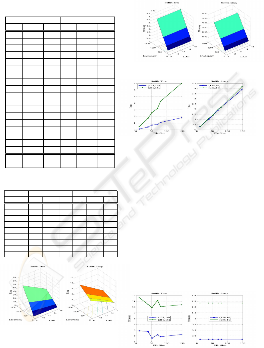
Table 3: Compression results for (Dictio-
nary,LAB)=(256,16).
ST SA
T M CR T M CR
1.3 4904 35.1 1.5 676 22.1
11.5 4932 38.2 10.0 676 27.4
9.0 5996 40.7 7.9 676 30.8
5.1 6388 36.1 4.9 676 24.4
0.8 4876 39.8 0.7 676 29.7
1.2 5044 40.2 1.1 676 30.2
0.7 5072 39.0 0.6 676 28.5
0.2 5044 40.1 0.2 676 30.0
0.2 5408 40.1 0.2 676 30.5
0.6 5352 41.2 0.5 676 32.0
0.5 6220 44.0 0.5 676 36.6
1.1 5296 49.1 1.0 676 45.4
0.7 5380 50.1 0.7 676 45.0
1.3 7228 42.8 1.3 676 33.2
2.3 5408 40.6 2.0 676 31.4
1.8 5044 39.7 1.6 676 30.0
0.3 5184 41.2 0.3 676 28.8
0.2 6080 50.5 0.2 676 47.0
2.2 5492 41.6 1.9 676 32.4
38.8 98856 35.0 12168
Table 4: Compression results for different lengths of dictio-
nary and LAB, over the set of 18 files listed in Table 1.
ST SA
(Dic,LAB) T M CR T M CR
(128,8) 3.6 5424 42.4 8.1 652 30.3
(128,16) 1.7 5440 43.3 3.9 660 32.5
(256,8) 15.3 11015 43.7 8.6 1292 39.0
(256,16) 7.1 11011 46.0 4.0 1300 41.6
(512,8) 34.4 21776 43.1 9.4 2572 43.6
(512,16) 15.8 21785 46.6 4.5 2580 46.7
(1024,8) 70.3 44136 41.9 11.1 5132 46.0
(1024,16) 32.8 44134 46.6 5.5 5140 49.6
(2048,32) 32.7 88856 46.5 4.5 10276 50.8
Figure 6: Encoding time (in seconds) as a function of the
length of the dictionary and the LAB, for ST and SA en-
coder.
Figure 7: Memory (in kB) as a function of the length of the
dictionary and the LAB, for ST and SA encoder.
Figure 8: Encoding time (in seconds) as a function of the
file size, for ST and SA encoder.
encoder the increase of the LAB from 8 to 16 low-
ers the encoding time. Figure 7 displays the ammount
of memory as a function of the length of the dictio-
nary and the LAB. The ammount of memory does not
change significantly with the length of the LAB. It in-
creases with the length of the dictionary; this increase
is higher for the ST encoder.
6.4 Dictionary of 128/256, LAB of 16
Selecting only a few files of different contents and
sizes, we narrow our analysis to following 6 files
(sorted by length): fields (11150 bytes), progc (39611
bytes), paper1 (53161 bytes), progl (71646 bytes), pa-
per2 (82199 bytes) and alice29 (152089 bytes). Fig-
ure 8 shows the encoding time for these files, with
dictionary of length 128 and 256 and a LAB of 16,
using ST and SA. For both encoders, we get a linear
Figure 9: Memory (in kB) as a function of the file size, for
ST and SA encoder.
SUFFIX ARRAYS - A Competitive Choice for Fast Lempel-Ziv Compressions
11

increase on the encoding time as the file size grows.
For the ST encoder, we get a larger increase.
Using the same files, we analyzed the amount of
memory required by both encoders. The results are
depicted in Figure 9, and their analysis leads us to
conclude that the SA encoder needs a much lower am-
mount of memory, that is the same for all files. The
ST encoder uses a variable ammount of memory and
the increase on the file size does not always imply an
increase on the necessary ammount of memory.
7 CONCLUSIONS
In this work, we have explored the use of suffix trees
(ST) and suffix arrays (SA) for the Lempel-Ziv 77
family of data compression algorithms, namely LZ77
and LZSS. The use of ST and SA was evaluated in
different scenarios, using standard test files of differ-
ent types and sizes. Naturally, we focused on the en-
coder side, in order to see how we could perform an
efficient search without spending too much memory.
A comparison between the ST and the SA encoders
was carried out, using the following metrics: encod-
ing time, memory requirement, and compression ra-
tio. Our main conclusions are:
• ST-based encoders require more memory than the
SA counterparts;
• the memory requirement of ST- and SA-based en-
coders is linear with the dictionary size; for the
SA-based encoders, it does not depende on the
contents of the file to be encoded;
• for small dictionaries, there is no significant dif-
ference in terms of encoding time and compres-
sion ratio, between ST and SA;
• for larger dictionaries, ST-based encoders are
slower that SA-based ones; however, in this case,
the compression ratio with ST is slightly better
than the one with SA.
These results support the claim that the use of SA
is a very competitive choice when compared to ST,
for Lempel-Ziv compression. We know exactly the
memory requirement of the SA, which depends on
the dictionary length. In application scenarios where
the length of the dictionary is large and the available
memory is scarce (e.g., a mobile device), it is prefer-
able to use SA instead of ST.
As future work, we intend to develop the SA en-
coder combining LCP and the simple accelerant and
supper accelerant (Gusfield, 1997, p´ag. 152, 153), to
speed up the search over the dictionary. This issue is
of greater importance for dictionaries of large dimen-
sions.
REFERENCES
Abouelhoda, M., Kurtz, S., and Ohlebusch, E. (2004). Re-
placing suffix trees with enhanced suffix arrays. Jour-
nal of Discrete Algorithms, 2(1):53–86.
Fiala, M. and Holub, J. (2008). DCA using suffix arrays. In
Data Compression Conference DCC2008, page 516.
Gusfield, D. (1997). Algorithms on Strings, Trees and Se-
quences. Cambridge University Press.
Karkainen, J., Sanders, P., and S.Burkhardt (2006). Linear
work suffix array construction. Journal of the ACM,
53(6):918–936.
Larsson, N. (1996). Extended application of suffix trees to
data compression. In Data Compression Conference,
page 190.
Larsson, N. (1999). Structures of String Matching and Data
Compression. PhD thesis, Department of Computer
Science, Lund University, Sweden.
Manber, U. and Myers, G. (1993). Suffix arrays: a new
method for on-line string searches. SIAM Journal on
Computing, 22(5):935–948.
McCreight, E. (1976). A space-economical suffix tree con-
struction algorithm. Journal of the ACM, 23(2):262–
272.
Sadakane, K. (2000). Compressed text databases with effi-
cient query algorithms based on the compressed suffix
array. In ISAAC’00, volume LNCS 1969, pages 410–
421.
Salomon, D. (2007). Data Compression - The complete ref-
erence. Springer-Verlag London Ltd, London, fourth
edition.
Sestak, R., Lnsk, J., and Zemlicka, M. (2008). Suffix array
for large alphabet. In Data Compression Conference
DCC2008, page 543.
Storer, J. and Szymanski, T. (1982). Data compression via
textual substitution. Journal of ACM, 29(4):928–951.
Ukkonen, E. (1995). On-line construction of suffix trees.
Algorithmica, 14(3):249–260.
Weiner, P. (1973). Linear pattern matching algorithm. In
14th Annual IEEE Symposium on Switching and Au-
tomata Theory, volume 27, pages 1–11.
Zhang, S. and Nong, G. (2008). Fast and space efficient
linear suffix array construction. In Data Compression
Conference DCC2008, page 553.
Ziv, J. and Lempel, A. (1977). A universal algorithm for
sequential data compression. IEEE Transactions on
Information Theory, IT-23(3):337–343.
SIGMAP 2008 - International Conference on Signal Processing and Multimedia Applications
12
