TIME DOMAIN ATTACK AND RELEASE MODELING

Applied to Spectral Domain Sound Synthesis

Cornelia Kreutzer, Jacqueline Walker

Department of Electronic and Computer Engineering, University of Limerick, Limerick, Ireland

Michael O’Neill

School of Computer Science and Informatics, University College Dublin, Dublin, Ireland

Keywords:

Audio Signal Processing, Spectral Music Synthesis, Modeling Real Instrument Sounds.

Abstract:

We introduce a time-domain model for the synthesis of attack and release parts of musical sounds. This

approach is an extension of a spectral synthesis model we developed: the Reduced Parameter Synthesis Model

(RPSM). The attack and release model is independent from a preceding spectral analysis as it is based on

the time domain sustain part of the sound. The model has been tested with linear and polynomial shaping

functions and produces good results for three different instruments. The time-domain approach overcomes the

problem of synthesis artifacts that often occur when using spectral analysis/synthesis methods for sounds with

transient events. Moreover, the model can be combined with any synthesis model of the sustain part and offers

the possibility to determine the duration of the attack and release parts of the sound.

1 INTRODUCTION

In the standard sinusoidal model used for speech

(McAuley and Quatieri, 1986) and musical sounds

(Serra, 1989; Serra and Smith, 1990), the harmonic

part of a given signal is modeled as a sum of sinu-

soidal components with time-varying amplitude, fre-

quency and phase. The remaining sound components

are then usually added to the model by using some

type of noise model. However, these methods are not

sufﬁcient to model transient parts of the signal. Tran-

sients mainly occur during the onset of a sound and

have long been known to be important for our per-

ception of timbre (Grey, 1977; McAdams and Cu-

nibile, 1992). A number of methods have been in-

troduced to provide a sinusoidal sound model that is

also capable of modeling transients more accurately.

Jensen (Jensen, 1999) proposed an amplitude model

in the frequency domain where the amplitude enve-

lope of each harmonic partial is ﬁtted with appropri-

ate functions. Verma and Meng (Verma and Meng,

2000) proposed an extension of the Spectral Modeling

Synthesis (SMS) framework to model transients by

performing sinusoidal modeling in the frequency do-

main. This is based on the observation that transient

components of a signal show the same behavior in

the frequency domain as sinusoidal components in the

time domain. Methods using exponentially damped

sinusoids to model transient events more accurately

have been proposed by (Nieuwenhuijse et al., 1998;

Boyer and Essid, 2002; Hermus et al., 2005). Meil-

lier and Chaigne (Meillier and Chaigne, 1991) applied

an autoregressive model which improved the spectral

analysis of percussive sounds compared to the stan-

dard FFT approach. In (Masri and Bateman, 1996)

the spectral analysis is improved by synchronizing

the analysis window to transient events. This over-

comes the problem that transient events, which occur

at a certain time, become diffused during the synthe-

sis process when using the standard sinusoidal model.

All these approaches focus on improving the si-

nusoidal sound model in the spectral domain. Thus,

the transient of the analyzed sound is captured more

accurately and artifacts during the synthesis process

are reduced. However, these interventions are inher-

ently limited in efﬁciency by the time-frequency un-

certainty principle.

In contrast to that, we propose a time domain

model for attack and release parts of musical sounds.

The model is combined with a spectral synthesis

model: the Reduced Parameter Synthesis Model

(RPSM) (Kreutzer et al., 2008). We model the sound

attack and release independently from a preceding

spectral analysis of these parts of the signal. There-

119

Kreutzer C., Walker J. and O’Neill M. (2008).

TIME DOMAIN ATTACK AND RELEASE MODELING - Applied to Spectral Domain Sound Synthesis.

In Proceedings of the International Conference on Signal Processing and Multimedia Applications, pages 119-124

DOI: 10.5220/0001936301190124

 SciTePress

fore, we exclude artifacts that might occur when us-

ing a transient analysis-synthesis model. These arti-

facts are due to interpolations of the sound partials

between signal frames when it comes to the synthesis

process. Our time domain approach in combination

with RPSM also leads to a reduction in computational

requirements, because it does not require us to model

the amplitude envelope of each partial individually in

detail.

2 REDUCED PARAMETER

SYNTHESIS MODEL

2.1 Frequency Estimation

To determine the frequency values within the synthe-

sis model we use a ﬂexible model that is not based

directly on a preceding spectral analysis but on the

basic knowledge about the sound. The fundamental

frequency, or pitch, as well as the number of har-

monic partials are user deﬁned values. This is par-

ticularly important if the synthesized sound lies out-

side the range of the instrument the model is supposed

to mimic. Also, within the range of an instrument

there is no restriction of the pitch value or the num-

ber of harmonics that can be chosen, since both val-

ues are entirely user deﬁned. Consequently we can

model whole tones, semitones or quarter tones of an

instrument as well as other notes whose pitch value is

anywhere in between or outside these tones.

We apply a random walk to several frequency par-

tials in order to reconstruct the naturalness of the

sound. Figure 1 (top) shows a representative result of

the SMS partial tracking algorithm (Amatriain et al.,

2002): in this particular case the result for a ﬂute note

(A4, played forte, non Vibrato (RWC, 2001, Instru-

ment Nr.33, Flute:Sankyo)). As illustrated, some of

the partials, especially the upper ones, show a certain

amount of variation or noisiness. Due to this nois-

iness a reconstruction of the sinusoidal parts of the

sound does keep the sound characteristics of the orig-

inal recording, although the residual part of the sig-

nal is neglected for the reconstruction. Based on this

observation we incorporate this noisiness into the si-

nusoidal partials of our synthesis model rather than

deﬁning a separate noise model. This is achieved by

the use of a one-dimensional random walk (Feller,

1968). A one-dimensional random walk can be de-

scribed as a path starting from a certain point, and

then taking successive steps on a one-dimensional

grid. The step size is constant and the direction of

each step is chosen randomly with all directions be-

100 200 300 400 500 600

2000

4000

6000

8000

10000

12000

Frame number

Frequency (Hz)

Harmonic partials − frequency tracks

0 100 200 300 400 500

2000

4000

6000

8000

10000

12000

Frame number

Frequency (Hz)

SynthModel: Harmonic partials − frequency tracks

Figure 1: SMS frequency analysis result of a ﬂute note

recording (A4 forte, non Vibrato (top) and estimated fre-

quency tracks for a note with 20 harmonics with the same

fundamental frequency (bottom).

ing equally likely.

For the purpose of our synthesis model random

walks are applied to certain harmonic partials in the

following way. First, the harmonic partials are di-

vided into three groups, where each group represents

a third of the overall number of harmonics. This

follows from the results of the SMS analysis which

shows different levels of variations for the lower, the

middle and the upper harmonics. Concerning the low-

est third of the harmonic partials - starting from the

fundamental frequency - no random walk is applied

as the analysis of these lower partials shows very lit-

tle variation. For the middle and the upper harmonic

partials a random walk is applied, where the starting

point of the random walk is determined by the basic

frequency of the harmonic partial. Basic frequency in

that case means the integer multiple of the fundamen-

tal frequency. Again, from the analysis result it can

be seen that the upper harmonics show more variation

than the middle ones. Due to that, and after testing

several levels of noisiness, the step size of the ran-

dom walk was set to 30 Hz for the upper harmonics

and to 15 Hz for the middle ones. Figure 1 (bottom)

shows the estimated frequency tracks for the synthe-

sis model compared to an SMS analysis result with

the same conditions (top).

SIGMAP 2008 - International Conference on Signal Processing and Multimedia Applications

120

2.2 Amplitude Estimation

In contrast to the frequency estimation which is not

directly taken from the sound analysis results, we use

SMS analysis results as a basis for estimating the am-

plitude values of the harmonic partials.

However, we reduce the number of parameters to

provide a ﬂexible synthesis model that is mostly inde-

pendent from the preceding sound analysis process.

This also reduces the computational complexity of

the synthesis process. Additionally, our main concern

is to keep the quality and naturalness of the musical

sound after the synthesis process in order to mimic

real instruments. Therefore, three different methods

have been applied to the analysis amplitude data. In

particular we have carried out amplitude estimation

by means of local optimization, lowpass ﬁlter estima-

tion and polynomial ﬁtting.

We start by applying a standard SMS analysis

(Amatriain et al., 2002) to obtain the amplitude pa-

rameters. To increase the number of spectral samples

per Hz and improve the accuracy of the peak detec-

tion process, we apply zero-padding in the time do-

main - using a zero-padding factor of 2. The STFT

was performed with a sampling rate of 44.1 kHz and a

Blackman-Harris window with a window size of 1024

points and a hop size of 256 points. From the resulting

frequency spectrum, 100 spectral peaks were detected

and subsequently used to track the harmonic partials

of the sound. The number of partials to be tracked

was set to 20. This analysis has been applied to sound

samples taken from the RWC database (RWC, 2001),

in particular to all notes over the range of a ﬂute, a

violin and a piano. Given the amplitude tracking re-

sults only one representative note for each instrument

has been chosen to provide the basis for the amplitude

values of the RPSM. However, this could be changed

in the future into using more than one amplitude tem-

plate, e.g., using different templates for the low notes

and the high notes within the range of an instrument.

2.2.1 Local Optimization

The SMS analysis provides one amplitude value for

each harmonic partial and for each frame of a given

sound signal. We reduce that parameter size by de-

termining the local maxima of each amplitude track.

This reduces the number of parameters to about a

third of the SMS analysis result. For example, for the

ﬂute note (A4, played forte, non Vibrato) the SMS

analysis consists of 12680 amplitude values. This is

reduced to 3015 values which represent all the local

maxima of the 20 harmonic partials.

We determine the local maxima of each amplitude

envelope by using the ﬁrst derivative of the amplitude

envelope function f

. Suppose we want to determine

if f

has a maximum at point x. If x is a maximum of

, then f

is increasing to the left of x and decreasing

to the right of x. The same principle applies for local

minima of f

. If x is a minimum of f

, then f

decreasing to the left of x and increasing to the right of

x. In contrast, if f

is increasing or decreasing on both

sides of x, then x is not a maximum or a minimum. In

terms of the ﬁrst derivative of f

this means, that f

increasing when the derivative is positive, and that f

is decreasing when the derivative is negative.

To compute the shape of each amplitude track,

necessary for the synthesis process, we then perform a

one-dimensional linear interpolation between the lo-

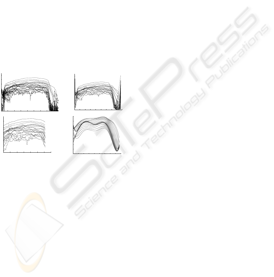
cal maxima of the track. Figure 2 (top right) illus-

trates an example of estimated amplitude tracks using

this approach as well as the SMS analysis results (top

left) for a violin note. As can be seen the shape of the

tracks are close to the SMS analysis result. However,

this is not the case for the attack and the release part

of the sound.

2.2.2 Lowpass Filter Estimation

The second curve ﬁtting method applied uses a low-

pass ﬁlter to estimate the overall amplitude envelope

of each partial. We apply a 3

order Butterworth low-

pass ﬁlter to the analysis data. We perform zero-phase

digital ﬁltering by processing the input data in both

the forward and reverse directions. After ﬁltering in

the forward direction, the ﬁltered sequence is reversed

and runs back through the ﬁlter. The resulting se-

quence has precisely zero-phase distortion and dou-

ble the ﬁlter order. As shown in Figure 2 (bottom left)

the envelope shapes of the estimated amplitude tracks

are similar to the local optimization estimation. How-

ever, the estimation takes signiﬁcantly longer to be

performed. Similar to the local optimization method,

no sufﬁcient estimate for the synthesis of the attack

and the release of the sound signal is obtained.

2.2.3 Polynomial Interpolation

Additionally we performed polynomial ﬁtting to ob-

tain an estimate for the several amplitude tracks. For

each amplitude envelope the coefﬁcients of a polyno-

mial of degree 6 are computed that ﬁt the data - in

our case the analysis result - in a least squares sense.

This computation is performed using a Vandermonde

matrix (Meyer, 2000)

V =







1 α

... α

n−1

1 α

... α

n−1

1 α

... α

n−1







(1)

TIME DOMAIN ATTACK AND RELEASE MODELING - Applied to Spectral Domain Sound Synthesis

121

since solving the system of linear equations Vu = y

for u with V being an n × n Vandermonde matrix is

equivalent to ﬁnding the coefﬁcients u

of the poly-

nomial

P(x) =

n−1

∑

j=0

(2)

of degree ≤ n − 1 with the values y

at α

(Meyer,

2000).

An example for the estimation result is shown in

Figure 2 (bottom right). Unlike the two other meth-

ods being used, the results are very smooth amplitude

envelopes. That is, all the small variations that can

be seen in the SMS analysis result are missing. Nev-

ertheless, the synthesized sounds preserve the timbre

of the particular instrument and the sound quality of

the original recordings. Regarding the ﬂute and the

violin, the polynomial estimation also gives a sufﬁ-

cient estimate for the attack and the release part of the

sound.

50 100 150 200 250 300 350 400

−100

−90

−80

−70

−60

−50

−40

−30

−20

−10

Frame number

Magnitude(dB)

Harmonic partials − amplitude tracks

0 50 100 150 200 250 300 350 400 450

−100

−90

−80

−70

−60

−50

−40

−30

−20

−10

Frame number

Magnitude(dB)

0 50 100 150 200 250 300 350

−80

−70

−60

−50

−40

−30

−20

Frame number

Magnitude(dB)

0 50 100 150 200 250 300 350 400 450

−110

−100

−90

−80

−70

−60

−50

−40

−30

Frame number

Magnitude(dB)

Figure 2: Violin note, A#3, forte, non vibrato: SMS am-

plitude analysis result, estimated amplitude tracks using lo-

cal optimization, LP ﬁlter estimation, and polynomial ﬁtting

(from top left to bottom right).

2.3 Spectral Synthesis

With the calculated frequency and amplitude parame-

ters we synthesize a new sound using an additive syn-

thesis method, which is based on spectral envelopes

and the inverse Fast Fourier Transform (Rodet and

Depalle, 1992). Compared to the traditional use of

oscillator banks for additive synthesis, this is a more

efﬁcient and faster approach.

3 TIME DOMAIN ATTACK AND

RELEASE MODELING

To improve the RPSM model in terms of sound at-

tack and release, we extend the synthesis model with a

time domain attack and release model. The approach

we are using corresponds to multiplying the sustain

portion of the sound by a time domain window. Thus,

we accomplish the desired transformation in the fre-

quency domain. This reduces the complexity of the

model signiﬁcantly, as the alternative is to map each

amplitude partial in detail through the attack and re-

lease stages in the frequency domain.

3.1 Linear Modeling

To synthesize the attack and release portions of the

sound we require the sustain part of the RPSM syn-

thesized signal in the time domain and the durations

of the attack and the release parts we want to model.

Both duration times may be user deﬁned and thus can

be changed according to the signal length and the in-

strument.

The attack is computed as follows. From the be-

ginning of the sustain signal we take a part with the

same length as the attack duration. This is the part

of the signal that is shaped to gain the attack portion.

Then, we carry out a point wise multiplication of this

part with a linear shaping function y

att

(n) = k ∗ x(n),

for n =

{

1,2,...,N

}

. This can be compared to the

application of a time domain window. The parame-

ters of y

att

are set according to the given signal, with

att

(1) = 0 to ensure that the sound starts at 0. The

length N of the shaping function is equal to the du-

ration of the attack. The slope k of the function is

determined by k = y

att

(N) − y

att

(1)/(N − 1). Thus,

att

(N) = 1. This allows for a smooth transition be-

tween the attack and the sustain portion of the sound

when they are joined.

For the release part of the sound the procedure is

similar to the attack, but here we perform the shap-

ing at the end of the sustain signal. From the end

of the sustain signal a part with the same length

as the release duration is taken. To compute the

sound release we carry out a point wise multiplica-

tion of this signal part with a linear shaping func-

tion y

rel

(m) = −k ∗ x(m), for m =

{

1,2,...,M

}

. The

function length M is equal to the duration of the re-

lease and y

rel

(M) = 0 to ensure that the sound ter-

minates to 0. The negative function slope k is deter-

mined by k = −y

att

(N) − y

att

(1)/(N − 1). To ensure

a smooth transition between the sustain and the re-

lease part of the sound the function parameters are set

so that y

rel

(1) = 0.5. Although setting y

rel

(1) = 0.5

works well for the three different instruments we have

tested so far, it must be noted that this value is largely

dependent on the shape of the given sustain signal.

After the computing attack and the release por-

tions, both are connected to the original sustain part

SIGMAP 2008 - International Conference on Signal Processing and Multimedia Applications

122

of the RPSM synthesized sustain signal. To do so,

the three separate waveforms are concatenated in the

order attack - sustain - release.

3.2 Polynomial Modeling

To obtain a more smooth and realistic attack and re-

lease, we also used a second order polynomial as a

shaping function. Setting the function parameters and

computing the particular attack and release signals

has been performed similarly to the linear shape.

To compute the attack a part of length N - equal

to the attack duration - is taken from the begin-

ning of the sustain signal. This waveform is then

point wise multiplied with the polynomial function

att

(n) = k ∗ x(n)

, for n =

{

1,2,...,N

}

. As with the

linear shaping function, the function parameters are

set to ensure y

att

(1) = 0 and y

att

(N) = 1 Therefore,

the sound starts at 0 and we gain a smooth transition

between the attack and the sustain portion of the syn-

thesized waveform.

For the sound release we also use a second or-

der polynomial, but this time with a negative slope.

From the end of the sustain signal a part of length

M - equal to the release duration - is taken. Subse-

quently, this waveform is point wise multiplied with

the polynomial function y

rel

(m) = −k ∗ x(m)

, for

m =

{

1,2,...,M

}

. The function parameters are set so

that y

rel

(1) = 0.5 and y

rel

(M) = 0. This provides for

a smooth transition between the sustain signal and the

release portion and ensures that the sound terminates

to 0. Again, note that the setting of y

rel

(1) depends on

the shape of the given sustain signal. For the instru-

ments we have tested so far, 0.5 has shown to be the

most suitable setting.

After computing the sound attack and the release,

both are connected to the original sustain part of the

RPSM synthesized sound to form the overall syn-

thesized time domain signal. The presented shaping

functions have produced good synthesis results for the

tested instruments. However, the method to determine

the shaping function for the attack and release model

could be further improved to overcome any possible

dependencies on the actual sound signal. Another

way to determine the parameters of the shaping func-

tion would be by modeling the shape of the release

component on the actual shape of the time domain

envelope.

4 EMPIRICAL EVALUATION

Figure 3 shows comparisons of the original sound

sample, the SMS synthesis result and the RPSM syn-

thesis result with the time-domain attack and release

for the three different instruments being used. In all

three cases the RPSM amplitude values have been

estimated using the local optimization method de-

scribed in Section 2.2.1. For the SMS results we ap-

plied a standard SMS analysis/synthesis (Amatriain

et al., 2002).

The presented RPSM model has been tested for

notes covering the whole range of a ﬂute (37 notes),

a violin (64 notes) and a piano (88 notes). An SMS

analysis has been carried out for all these notes us-

ing recorded samples from the RWC database (RWC,

2001). The analysis was done to ﬁnd a representa-

tive note for the presented amplitude model and to

compare the synthesis results obtained by our model

with the standard SMS results. The frequency esti-

mation works well and allows a large ﬂexibility when

choosing the fundamental frequency. Due to the ran-

dom walk that is applied to higher frequency partials

the synthesized sound keeps the natural noisiness of

the real instrument recording without the need for a

separate noise model. Concerning the three different

amplitude estimation methods, all of them perform

well when estimating the sustain part of the signal.

Although, only the polynomial ﬁt gives a satisfac-

tory estimate for the attack and the release parts of

the signal at the same time. The combination of the

basic RPSM model with the time domain attack and

release model overcomes these difﬁculties and pro-

vides an efﬁcient method to model the beginning and

the end of the sound. Moreover, the attack/release

model is independent from a preceding spectral anal-

ysis and from the computation of the sustain portion

of the sound. Using this approach we avoid artifacts

that result from smoothing transient events, a problem

connected with spectral transient analysis/synthesis

methods. Together with the user deﬁned duration, the

new approach presented here allows for a ﬂexible syn-

thesis model.

5 CONCLUSIONS

We introduced a time domain attack and release

model as a an extension of a Parametric Synthesis

Model for musical sounds. To obtain the shape of the

note onset and release we use linear and polynomial

shaping functions. The RPSM model has been tested

for notes covering the whole range of three different

instruments; a ﬂute, a violin and a piano.

Future work will be focused on analyzing the ef-

fects of the time domain model on the spectral repre-

sentation of the signal and using the actual sound en-

velope for shaping the sound attack and decay. More-

TIME DOMAIN ATTACK AND RELEASE MODELING - Applied to Spectral Domain Sound Synthesis

123

0 0.2 0.4 0.6 0.8 1 1.2 1.4 1.6 1.8 2

x 10

−0.2

0.2

Original sound sample

0 2 4 6 8 10 12 14 16 18

x 10

−0.2

0.2

SMS synthesis result

0 2 4 6 8 10 12 14 16

x 10

−1

PSM plus linear attack/release synthesis result

0 2 4 6 8 10 12 14 16

x 10

−1

PSM plus polynomial attack/release synthesis result

0 2 4 6 8 10 12 14

x 10

−0.2

0.2

Original sound sample

0 2 4 6 8 10 12

x 10

−0.2

0.2

SMS synthesis result

0 2 4 6 8 10

x 10

−1

PSM plus linear attack/release synthesis result

0 2 4 6 8 10

x 10

−1

PSM plus polynomial attack/release synthesis result

0 5 10 15

x 10

−0.5

0.5

Original sound sample

0 2 4 6 8 10 12 14

x 10

−0.5

0.5

SMS synthesis result

0 2 4 6 8 10 12

x 10

−1

PSM plus linear attack/release synthesis result

0 2 4 6 8 10 12

x 10

−1

PSM plus polynomial attack/release synthesis result

Figure 3: Time domain plots of original sound, SMS result and RPSM result with attack/release model(from left to right:

ﬂute, violin, piano).

over, we are going to perform listening tests to gain

detailed results for a comparison between the original

recorded sound samples, SMS synthesis results and

the presented RPSM model.

ACKNOWLEDGEMENTS

This work was supported by the Science Foundation

Ireland (SFI) under the National Development Plan

(NDP) and Strategy for Science Technology & Inno-

vation (SSTI) 2006-2013.

REFERENCES

Amatriain, X., Bonada, J., Loscos, A., and Serra, X. (2002).

Spectral Processing in DAFx – Digital Audio Effects,

chapter 10, pages 373–439. edited by Udo Zoelzer.

John Wiley & Sons.

Boyer, R. and Essid, S. (2002). Transient Modeling

with a Frequency–Transform Subspace Algorithm and

”Transient+Sinusoidal” Scheme. pages 865–868,

vol.2. IEEE International Conference on Digital Sig-

nal Processing (DSP). Thera, Greece.

Feller, W. (1968). Introduction to Probability Theory and

its Applications. Wiley series in probability and math-

ematical statistics. John Wiley & Sons, 3rd edition.

Grey, J. M. (1977). Multidimensional Perceptual Scaling of

Musical Timbre. Journal of the Acoustical Society of

America, 61(5):1270–1277.

Hermus, K., Verhelst, W., Lemmerling, P., Wambacq, P.,

and van Huffel, S. (2005). Perceptual Audio Mod-

eling with Exponentially Damped Sinusoids. Signal

Processing, 85(1):163–176. Elsevier North-Holland,

Inc., Amsterdam, The Neatherlands.

Jensen, K. (1999). Timbre Models of Musical Sounds. PhD

thesis, University of Copenhagen, Copenhagen, Den-

mark.

Kreutzer, C., Walker, J., and O’Neill, M. (2008). A Para-

metric Model for Spectral Sound Synthesis of Musi-

cal Sounds. International Conference on Audio, Lan-

guage and Image Processing (ICALIP). Shanghai,

China.

Masri, P. and Bateman, A. (1996). Improved Modelling

of Attack Transients in Music Analysis–Resynthesis.

pages 100–103. International Computer Music Con-

ference (ICMC), IEEE. Hong Kong, China.

McAdams, S. and Cunibile, J.-C. (1992). Perception of Tim-

bral Analogies. Physical Transactions of the Royal

Society, 336. Series B.

McAuley, R. and Quatieri, T. (1986). Speech Analy-

sis/Synthesis Based on a Sinusoidal Representation.

34:744–754. IEEE Transactions on Acoustics, Speech

and Signal Processing.

Meillier, J.-L. and Chaigne, A. (1991). AR Modeling of

Musical Transients. pages 3649–3652. IEEE Inter-

national Conference on Acoustics, Speech and Signal

Processing (ICASSP). Toronto, Canada.

Meyer, C. (2000). Matrix Analysis and Applied Linear Al-

gebra, chapter 4. SIAM, Philadelphia, PA.

Nieuwenhuijse, J., Heusdens, R., and Deprettere, E. (1998).

Robust Exponential Modeling of Audio Signals. pages

3581–3584. IEEE International Conference on Acous-

tics, Speech and Signal Processing (ICASSP). Seattle,

Washington, USA.

Rodet, X. and Depalle, P. (1992). Spectral Envelopes and

Inverse FFT Synthesis. 93rd AES Convention, San

Francisco, AES Preprint No. 3393 (H-3).

RWC (2001). Real World Computing (RWC) Music

Database – Musical Instrument Sound. RWC–MDB–

I–2001 No. 01–50, Tokyo, Japan.

Serra, X. (1989). A System for Sound Analy-

sis/Transformation/Synthesis based on a Determinis-

tic plus Stochastic Decomposition. PhD thesis, Stan-

ford University.

Serra, X. and Smith, J. (1990). Spectral Modeling Synthe-

sis:A Sound Analysis/Synthesis Based on a Determin-

istic plus Stochastic Decomposition. Computer Music

Journal, 14(4):12–24.

Verma, T. S. and Meng, T. H. Y. (2000). Extending Spectral

Modeling Synthesis with Transient Modeling Synthe-

sis. Computer Music Journal, 24(2):47–59.

SIGMAP 2008 - International Conference on Signal Processing and Multimedia Applications

124