
PARTIAL TRACKING IN SINUSOIDAL MODELING
An Adaptive Prediction-based RLS Lattice Solution
Leonardo O. Nunes, Paulo A. A. Esquef, Luiz W. P. Biscainho and Ricardo Merched
LPS - DEL/Poli & PEE/COPPE, Federal University of Rio de Janeiro, Rio de Janeiro, Brazil
Keywords:
Acoustical signal processing, Sinusoidal modeling, Partial tracking, Linear prediction, Adaptive filtering, Lat-
tice filters.
Abstract:
Partial tracking plays an important role in sinusoidal modeling analysis, being the stage in which the model
parameters are obtained. This is accomplished by coherently grouping the spectral peaks found in each frame
into time-evolving tracks of varying frequency and amplitude. The main difficulties faced by partial tracking
algorithms are the analysis of polyphonic signals and the pursuit of tracks exhibiting strong modulations in
frequency and amplitude. In these circumstances, linear prediction over the trajectory of a given track has
been shown to improve partial tracking performance. This paper proposes an adaptive RLS lattice filter for
the purpose of prediction in partial tracking. A new heuristic which certifies the filter convergence is also
presented. Computer simulation results are shown to compare the proposed implementation with that of other
predictors. The performance of the proposed solution is similar to that of competing methods, albeit with
reduced computational complexity as well as improved numerical stability.
1 INTRODUCTION
Audio signals are predominantly resonant in nature,
being thus well described by a sum of amplitude- and
frequency-modulated sinusoids. Taking advantage of
that fact, sinusoidal modeling (SM) has been intro-
duced for speech analysis in (McAulay and Quatieri,
1986) and for audio signals in (Smith III and Serra,
1987), being later expanded (Serra, 1997) and modi-
fied (George and Smith, 1992) to suit various audio-
related applications, such as speech synthesis and
modifications, musical instrument synthesizers, audio
coding, and automatic transcription of music.
The classical MQ sinusoidal analysis algorithm
presented in (McAulay and Quatieri, 1986) can be di-
vided into two separate steps. First, the sinusoidal
components are detected on a frame-by-frame basis,
usually by peak picking from the magnitude spectrum
of the signal computed via the Short-Time Fourier
Transform. The detected peaks are then linked
across the frames to form the partial tracks. Each
track, if correctly detected, models an amplitude- and
frequency-modulated sinusoid.
The main difficulties faced by a partial tracking al-
gorithm are in robustly estimating the trajectory of a
partial that exhibits strong frequency modulation (vi-
brato) and/or amplitude modulation (tremolo), as well
as in resolving partial ambiguities that may occur dur-
ing analysis of a polyphonic audio recording.
Several proposals have been made in attempt to
improve partial tracking performance. In (Depalle
et al., 1993) hidden Markov models, along with a
Viterbi algorithm, are used to model the track trajec-
tory in order to achieve optimum track continuation.
Kalman filters have also been considered in (Sterian
and Wakefield, 1998) for modeling the tracks’ behav-
ior of musical instrument sounds, provided knowl-
edge of a model for the instrument being analyzed.
Another approach for partial tracking makes use of
autoregressive modeling to predict the evolution of
the track parameters over time. In (Lagrange et al.,
2003) a predictor based on the Burg’s method has
been shown to be quite effective for such task, spe-
cially in situations where crossing frequency trajecto-
ries occur. In (Nunes et al., 2007b) an adaptive-filter
solution is described for the prediction of the partial
tracks. The sequential nature of adaptive filters has
been demonstrated to be specially suited for the pre-
diction problem at hand.
This work presents an RLS lattice filter solution to
the prediction of the frequency and amplitude compo-
nents of a given partial track. The proposition, which
builds on a previous solution (Nunes et al., 2007b), at-
tains similar performancebutwith a reduction in com-
84
O. Nunes L., A. A. Esquef P., W. P. Biscainho L. and Merched R. (2008).
PARTIAL TRACKING IN SINUSOIDAL MODELING - An Adaptive Prediction-based RLS Lattice Solution.
In Proceedings of the International Conference on Signal Processing and Multimedia Applications, pages 84-91
DOI: 10.5220/0001937000840091
Copyright
c
SciTePress

putational complexityfrom O (n
2
) to O (n). Moreover,
a heuristic that discards unrealistic predictions during
the filter’s training period is also described.
After this introduction, Section 2 briefly outlines
the processing stages involved in SM analysis, de-
scribing the standard MQ partial tracking algorithm,
and reviewing the adaptive filter framework for the
problem. In Section 3, the proposed lattice filter
solution is introduced. Computer simulation results
that illustrate the performance of the proposed pre-
dictor are shown in Section 4. Finally, conclusions
are drawn.
2 SINUSOIDAL ANALYSIS
OVERVIEW
Sinusoidal modeling (McAulay and Quatieri, 1986)
describes an audio signal x(t) as a sum of L sinusoids,
i.e.,
x(t) =
L
∑
l=1
A
l
(t)sin(Ψ
l
(t)), (1)
with
Ψ
l
(t) = Ψ
l
(0) +
Z
t
0
ω
l
(u)du, (2)
where A
l
(t) is the modulated amplitude and Φ
l
(t) is
the modulated phase of partial l. In practice, Eq. (1)
is commonly replaced by a discrete model,
x[n] =
L
∑
l=1
A
l
[n]sin(Ψ
l
[n]). (3)
For a given partial l, the approximations A
l
[n] ≈ A
l
and Ψ
l
[n] ≈ Ω
l
n + Ψ
l
[0], where A
l
and Ω
l
are con-
stant values, hold true within a sufficiently short N-
sample frame.
The main objective of a sinusoidal analysis al-
gorithm consists in estimating A
l
and Ω
l
across the
frames. The typical stages (Serra and Smith III, 1990)
involved in the analysis portion of an SM system are
illustrated in Fig. 1.
Decomposition
Time/Frequency
Partial
Detection
Peak
x[n]
Tracks
Tracking
Partial
Figure 1: Processing stages of a sinusoidal analysis system.
The ‘time / frequency decomposition’ stage com-
putes the discrete-time Short-Time Fourier Transform
of the audio signal x[n], i.e.,
X[m,k] = STFT(x[n,m])
=
1
N
N−1
∑
n=0
w[n]x[n+ mH]e
− jk
2π
N
n
,
(4)
where w[n] is a window function of length N, e.g. the
Hamming window, k is the frequency bin index, m is
the frame index, and H is the frame hop (in samples)
along time. Out of X[m, k], the ‘peak detection’ stage
is supposed to select only those peaks that correspond
to stationary sinusoidal components present in frame
m. If desired, precise estimates for the amplitude and
frequency of the detected peaks can be obtained by
a number of dedicated methods (Lagrange and Marc-
hand, 2007). Finally, the partial tracking is responsi-
ble for coherently grouping peaks across consecutive
frames into the so-called partial tracks.
2.1 McAulay & Quatieri Algorithm
The objective of this section is twofold: to describe
the MQ algorithm, which will be extended in the next
section ,and else, to illustrate the difficulties that arise
in the partial tracking problem.
The MQ algorithm, proposed in (McAulay and
Quatieri, 1986) for speech analysis and adapted to au-
dio signals in (Smith III and Serra, 1987), is consid-
ered the standard algorithm for partial tracking and
serves as a starting point to many algorithms found in
the literature.
The MQ algorithm is summarized below:
1. To each track i in frame m with corresponding
peak frequency f
i
[m], the closest peak p, with fre-
quency f
p
[m + 1] such that | f
p
[m + 1] − f
i
[m]| ≤
∆f, isassigned by the algorithm. When two tracks
dispute the same peak, the one with the clos-
est frequency wins the conflict. The other track
searches for the next closest peak.
2. An emerging track is created to accommodate any
unassigned peaks. If a track stays in the emerg-
ing state for more than E frames, its state changes
to evolving. If an emerging track does not find a
continuation after E frames, it is then discarded.
3. If in frame m + 1 a track does not find any peak,
it is assigned a vanishing status, and its current
amplitude-frequencypair is propagated to the next
frame. If a track finds a continuation in at least S
frames, it leaves the vanishing state, being other-
wise considered inactive.
The algorithm performance is strongly dependent
on the choice of parameters {∆ f,E,S}. The role of
each parameter in the algorithm is described below:
• The ∆f parameter controls the maximum fre-
quency variation allowed and is usually frequency
dependent. For instance, ∆f = 0.03f
i
[m] is a com-
mon choice, since it corresponds to a quarter-tone
variation around f
i
[m].
PARTIAL TRACKING IN SINUSOIDAL MODELING - An Adaptive Prediction-based RLS Lattice Solution
85

• The E parameter is responsible for removing short
tracks, possibly formed by wrongly identified
peaks.
• The S parameter avoids track discontinuation as a
consequence of missing peaks.
The above procedure can fail to correctly identify
a track continuation in signals with vibrato or poly-
phonic audio. The occurrence of vibrato can lead to
a large frequency variation between adjacent frames,
requiring thus a too permissive choice for the ∆ f pa-
rameter. On the other hand, in polyphonic signals,
the occurrence of closely spaced track trajectories in
frequency (and even crossing frequency trajectories)
demands a very stringent choice of ∆f. Moreover, by
only considering the frequency evolution of the tracks
the MQ tracker ignores the preservation of the ampli-
tude continuity, which can lead to audible artifacts in
the re-synthesized signal.
The solution presented in the next section aims
at circumventing some of the aforementioned prob-
lems. By using previously acquired track information
to predict the frequency trajectory and comparing the
predicted with the observed peak value, the ∆ f pa-
rameter can be set to a small value even for tracks
with significant frequency variations, thus favoring a
better performance in the polyphonic case. Prediction
can also be made for the track amplitude information
to better select a continuation of a given track. All
these modifications make the algorithm more robust
in the sense that a single set of well-tuned processing
parameters suffices to the purpose of partial tracking
for a wider class of signals.
2.2 Prediction-based Partial Tracking
A rather natural extension to the MQ algorithm is ob-
tained by using predicted values for frequency and
amplitude of a given track, instead of using their last
measured values (Lagrange et al., 2007). This way,
the information acquired up to a determined frame is
used to obtain the best continuation for the track.
Figure 2 depicts a prediction-based partial track-
ing algorithm, which works as follows: for a given
track i, the most prominent spectral peaks of the sig-
nal at frame m (stored in amplitude-vector A[m] and
frequency-vector f[m]) are compared with predicted
values of amplitude (
ˆ
A
i
[m]) and frequency (
ˆ
f
i
[m]);
then a decision heuristics, to be discussed later, se-
lects amplitude
A
i
[m] and frequency f
i
[m] as the best
track continuation path.
The predicted values are obtained by minimizing
a function of the error between the estimated and the
“real” values of the peaks parameters. Since this min-
imization is performed sequentially on the track data,
Decider
A[m]
f [m]
f
i
[m − 1]
A
i
[m − 1]
e
i
[m]
ˆ
f
i
[m]
A
i
[m]
f
i
[m]
ˆ
A
i
[m]
Predictor
Figure 2: Prediction scheme for track i at frame m.
the model can be adapted whenever a new input sam-
ple (new peak assigned to a given track) is fed to the
predictor.
In (Nunes et al., 2007b), a regularized recursive
least-squares procedure is proposed for sequentially
predicting the amplitude and the frequency of each
partial. Defining the output vector with the predicted
parameters of the ith track by y
i
[m] =
ˆ
A
i
[m]
ˆ
f
i
[m]
and the input vector with the past J known parameters
by x
i
[m] =
h
A
T
i
[m− 1]
f
T
i
[m− 1]
i
, with
A
i
[m− 1] =
A
i
[m− 1]
A
i
[m− 2] · · · A
i
[m− J]
T
(5)
f
i
[m− 1] =
f
i
[m− 1] f
i
[m− 2] ··· f
i
[m− J]
T
, (6)
one can write
y
i
[m] = x
i
[m]W
i
[m− 1], (7)
where W
i
[m] is a 2J × 2 coefficient-matrix.
Given a choice of α > 0 and a forgetting factor
0 << λ ≤ 1, the exponentially-weighted regularized
least-squares problem (Sayed, 2003) seeks the matrix
W
i
[m] that minimizes
λ
m+1
W
T
i
[m]P
−1
J
W
i
[m]
+
m
∑
l=0
λ
m−l
kd
i
[l] − x
i
[l]W
i
[m]k
2
, (8)
where d
i
[m] =
A
i
[m] f
i
[m]
is the desired-signal
vector and P
−1
J
= α
−1
I
J
, with I
J
denoting a Jth-order
identity matrix.
Referring to Figure 2 again, the predicted ampli-
tude and frequency values at frame m are used to
choose the best track continuation from the parame-
ter vector (A and f) of the detected peaks. The chosen
track continuations,
A[m] and f[m], are then employed
to update the coefficient-matrix to time m. This new
coefficient-matrix, in conjunction with the updated
input-vector x[m+ 1], is used to predict the amplitude
and frequency values for the track at frame m+ 1.
The decision strategy adopted in (Nunes et al.,
2007b) is similar to that described in Section 2.1 and
to the method proposed in (Lagrange et al., 2007).
During the first qJ frames, q ≥ 1, the predicted results
are simply discarded while the filter is trained. For an
SIGMAP 2008 - International Conference on Signal Processing and Multimedia Applications
86

evolving track, given the vectors containing the pa-
rameters of detected peaks, f[m] and A[m], the candi-
date peaks are selected such that |
ˆ
f
i
[m]− f
p
[m]| ≤ ∆ f,
where i is the track index and p is the peak index. The
distance
|
ˆ
f
i
[m] − f
p
[m]|
ˆ
f
i
[m]
+ κ
|
ˆ
A
i
[m] − A
p
[m]|
ˆ
A
i
[m]
(9)
is calculated for all peak candidates and the one
nearest to its predicted counterpart is appended to the
track trajectory. The treatment of emerging and van-
ishing tracks follows the guidelines already described
in Section 2.1.
The aforementioned scheme considers both am-
plitude and frequency information into their joint pre-
diction. However, depending on the type of sound
source, or even on the level of noise contamination,
the track amplitude may behave more unpredictably
than the corresponding frequency, thus impairing the
estimation of the latter. For these cases, an alternative
uncoupled structure can be straightforwardly obtained
with two separate predictors, one for the frequency
and another for the amplitude of the tracks.
Next, an RLS lattice filter is presented as a solu-
tion to the prediction problem with an accompanying
decision heuristic.
3 LATTICE FILTER SOLUTION
The adaptive filter described in the previous Section
can be considered as a fixed order algorithm in the
sense that only time updates are performed in the fil-
ter. Thus, only quantities related to the solution of
a fixed order prediction are propagated. The lattice
solution, on the other hand, uses both time and or-
der recursions (up to a predefined order) to obtain the
predicted values by sequentially solving linear predic-
tion problems of increasing order. The solution thus
obtained exhibits several advantages over the previ-
ous algorithm, including improved numerical behav-
ior, stability, and reduced computational complex-
ity (Sayed, 2003).
The notation used so far has to be adapted due to
the order-recursivenature of the lattice filter. An addi-
tional sub-index j, denoting the jth-order solution for
a given quantity will be used throughout this section.
In this work, an a priori lattice filter is employed
to predict the frequency and amplitude of the tracks.
This is equivalent to the uncoupled version of the
prediction scheme described in Section 2.2. Thus,
given a choice of α > 0 and of a forgetting factor
0 << λ ≤ 1, the lattice filter obtains the weight vector
w
i,J
[m] that minimizes the following Jth-order least-
squares cost function (Sayed, 2003):
λ
m+1
w
i,J
[m]
T
P
−1
J
w
i,J
[m]
+
m
∑
l=0
λ
m−l−1
d
i
[l] − x
T
i
[l]w
i,J
[m]
2
, (10)
where, in this case, x
i
[m] can be either
A
i
[m − 1],
for the amplitude predictor, or f
i
[m − 1], for the fre-
quency predictor. d
i
[m] is the desired signal at time
m, which can be either A
i
[m] or f
i
[m], accordingly,
whereas P
−1
J
= α
−1
diag{λ
−2
,λ
−3
,··· , λ
−(J+1)
} is a
regularization matrix. The solution of order j for the
ith track at frame m can be obtained through the fol-
lowing equations:
ζ
f
i, j
[m] = λζ
f
i, j
[m− 1] + α
2
i, j
[m]γ
i, j
[m− 1]
ζ
b
i, j
[m] = λζ
f
i, j
[m− 1] + β
2
i, j
[m]γ
i, j
[m]
δ
i, j
[m] = λδ
i, j
[m− 1] + α
i, j
[m]β
i, j
[m− 1]γ
i, j
[m− 1]
ρ
i, j
[m] = λρ
i, j
[m− 1] + e
i, j
β
i, j
[m]γ
i, j
[m− 1]
β
i, j+1
[m] = β
i, j
[m− 1] − κ
b
i, j
[m− 1]α
i, j
[m]
α
i, j+1
[m] = α
i, j
[m] − κ
f
i, j
[m− 1]β
i, j
[m− 1]
e
i, j+1
[m] = e
i, j
[m] − κ
i, j
[m− 1]β
i, j
[m]
γ
i, j+1
[m] = γ
i, j
[m] − (γ
i, j
[m]β
i, j
[m])
2
/ζ
b
i, j
[m]
κ
b
i, j
[m] = δ
i, j
[m]/ζ
f
i, j
[m]
κ
f
i, j
[m] = δ
i, j
[m]/ζ
b
i, j
[m− 1]
κ
i, j
[m] = ρ
i, j
[m]/ζ
b
i, j
[m]
with γ
i,0
[m] = 1, β
i,0
[m] = α
i,0
[m] = x
i
[m] and e
i,0
[m] =
d
i
[m]. Hence the solution at frame m can be calcu-
lated by iterating the equations above for j varying
from 0 up to the desired predictor order J. The time
initialization of these quantities is described later in
this section.
As can be seen, the lattice filter does not explicitly
find the optimum weight vector. Both weight vector
and predicted values could be computed through ad-
ditional recursions along the adapting procedure. A
simple solution is adopted here to compute only the
predicted value after a given time-update of the filter.
For this, the key quantity is the a priori error of the
filter, defined as
e
i,J
[m] = d
i
[m] − x
T
i
[m]w
i
[m− 1]. (11)
The predicted value for frame m can be written as
y
i
[m] = x
T
i
[m]w
i
[m− 1], (12)
where y
i
[m] can be either
ˆ
A
i
[m] or
ˆ
f
i
[m], leading to
y
i
[m] = −e
i,J
[m]|
d
i
[m]=0
. (13)
Hence, in order to obtain the predicted value from
the filter at frame m, a new quantity, numerically
PARTIAL TRACKING IN SINUSOIDAL MODELING - An Adaptive Prediction-based RLS Lattice Solution
87

equal to the a priori error with a null desired signal, is
used. This way, the predicted value can be calculated
through the following order-update recursions:
α
i, j+1
[m] = α
i, j
[m] − κ
f
i, j
[m− 1]β
i, j
[m− 1]
β
i, j+1
[m] = β
i, j
[m− 1] − κ
b
i, j
[m− 1]α
i, j
[m]
y
i, j+1
[m] = y
i, j
[m] + κ
i, j
[m− 1]
β
i, j
[m],
with y
i,0
[m + 1] = 0 and
β
i,0
[m] = α
i,0
[m] initialized
either as
A[m − 1] or f[m− 1]. Notice that all quan-
tities involved in this calculation are available at time
m− 1, after the corresponding time-update of the lat-
tice filter.
Another issue with the prediction-based partial
tracker is the filter convergence. Partial tracking per-
formance may be hindered if prediction comes from a
filter whose convergence has not yet been achieved.
In order to overcome this limitation the following
heuristic is proposed: if the distance from the pre-
dicted value to the last element in the data vector is
too large, the predicted value is ignored and the last
element is used as the predicted value. This criterion
guarantees that the predicted values of frequency and
amplitude being used for comparison are always close
to those of the track parameters, thus avoiding discon-
tinuities in the obtained tracks.
The decision algorithm follows that of Section 2.2
with some modifications. The function used to decide
over a valid track is defined by Eq. (9). The main
change is on the handling of missing peaks. If a track
i does not find a suitable peak in frame m, it takes the
predicted amplitude and frequency. However, in the
next frame, a modified two-step ahead predictor used;
in other words, the amplitude and frequency in frame
m+ 1 are predicted using the information up to frame
m− 1. If in the next frames the track still does not find
a continuation, the same modified scheme proceeds.
Formally, if a track is in the vanishing state during s
consecutive frames and remains in it at frame m, the
following predictor is used,
y
i
[m] = x
T
i
[m− s] ˜w
i
[m− s− 1], (14)
where the prediction coefficients are found by min-
imizing the cost function in Eq. (10) with d
i
[m] =
x
i
[m + 1]. This way, the optimum predicted value is
always used to search a track continuation, given the
available track information.
When a peak is not selected to continue any track,
a new track is created to accommodate the peak.
The predictor for this new track has to be initialized
with the following values: γ
i, j
[−1] = 1, δ
i, j
[−1] =
0 = ρ
i, j
[−1] = β
i, j
[−1] =
β
i, j
[−1] = α
i, j
[−1] = 0,
κ
f
i, j
[−1] = κ
b
i, j
[−1] = κ
i, j
[−1] = 0, ζ
f
i, j
= α
−1
λ
−2
, and
ζ
b
i, j
[−1] = α
−1
λ
− j−2
; for j from 0 up to J −1. This is
the necessary time initialization mentioned earlier. As
can be noted, the lattice filter does not need any ma-
trix structure, which reduces the memory use of the
algorithm in relation to the RLS solution.
The parameters of the lattice filter are the predic-
tor order J, the forgetting factor λ, and the regulariza-
tion factor α. The value of J is usually larger than 2
and not bigger than 10 (Lagrange et al., 2007). Al-
though a larger J favors lowering the prediction error,
it may imply an undesirably longer training period for
the filter. Setting 2 ≤ J ≤ 6 for both the amplitude and
the frequency predictors has been shown to be a good
compromise between the two conflicting goals above.
The forgetting factor controls how much the past sam-
ples influence the prediction. Adopting λ close to
0.98 has been found to be adequate for the predic-
tion of tracks. The α parameter controls how much
the regularization affects the prediction. A high value
of α (around 2000) allows the regularization factor to
be quickly forgotten. On the other hand, if the pre-
diction coefficients are known to vary little from the
initial estimate (as is the case in this paper) a small α
helps speeding up filter convergence.
It should be noted that the frequency values of
a given track usually drift around a fixed center-
frequency. Considering this frequency in the pre-
diction can slow down filter convergence, impairing
tracking performance. To avoid that, in the proposed
system the track frequency prediction is always car-
ried out relative to the frequency firstly attributed to a
given track.
4 COMPUTER SIMULATIONS
This section is devoted to investigate the performance
of the proposed adaptive lattice predictor in compari-
son with a few other predictors found in the literature.
It also illustrates how the partial trackers behavewhen
analyzing natural audio signals.
4.1 Example 1: Test Setup
The first experiment is meant to assess the perfor-
mance of three predictors: the predictor based on
Burg’s method presented in (Lagrange et al., 2007),
the RLS predictor described in Section 2.2, and the
lattice predictor detailed in Section 3. For both the
RLS and lattice predictors λ = 0.98 and α = 10 have
been adopted. For the Burg predictor the length of
the observation window was chosen to be equivalent
to the duration (in samples) for which the exponential
window of the previous methods convey 90% of its
SIGMAP 2008 - International Conference on Signal Processing and Multimedia Applications
88
energy (Laakso and V¨alim¨aki, 1998). The prediction
order of all methods was chosen as 4.
The artificial frequency track depicted in Figure 3,
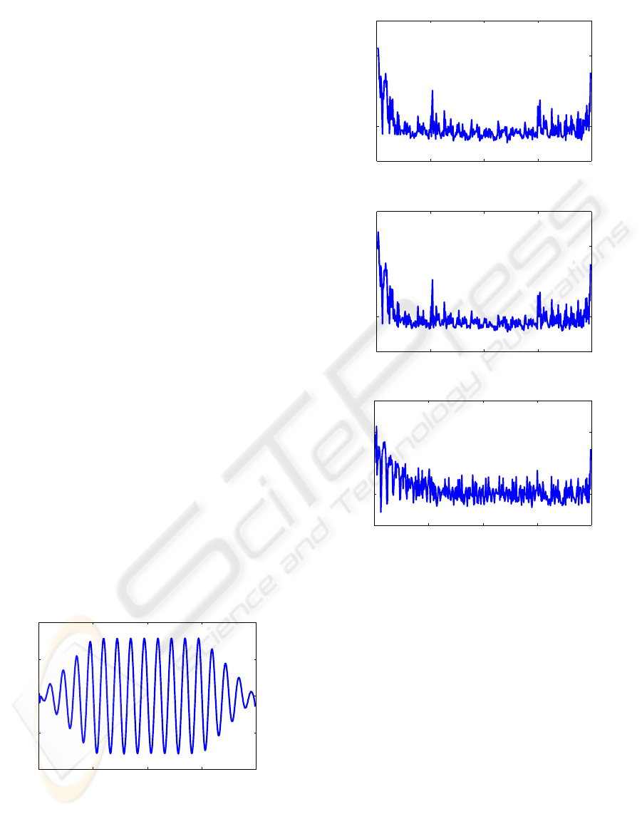
which simulates the behavior of a partial from a tone
played with vibrato, has been used as a test signal. It
consists of a frequency variation of sinusoidal nature,
centered around 440 Hz, with rate equal to 0.25 rad/s,
and amplitude depth of ±7 Hz multiplied by a trape-
zoidal envelope. White Gaussian noise was summed
to this signal so as to force an SNR equal to 40 dB.
4.2 Example 1: Results
The mean squared prediction error (MSE) of each
method is displayed in Figure 4. As can be seen,
the performance of the RLS and lattice methods was
equivalent, except for the initial parts of the MSE
curves, which differ due to the use of different reg-
ularization matrices in each case. The Burg predictor
yielded larger MSE and variance, being poorer in per-
formance.
According to this first experiment, both the RLS
and lattice prediction filters have similar performance,
mainly due to the minimization of the same cost func-
tion. The difference between them is in the compu-
tational complexity requirements. The RLS solution
has an asymptotic computationalcomplexity of O (J
2
)
as opposed to O (J) of the proposed lattice solution,
where J stands for prediction order. Since the number
of active filters is proportional to the number of active
tracks in a given frame, the aforementioned reduction
in computational cost can have a great impact on the
overall processing load of a sinusoidal analysis sys-
tem. Moreover, the quantities that need to be saved
for each filter between adjacent frames are reduced in
the lattice filter, leading to less memory use.
0 100 200 300 400
430
435
440
445
450
Time (samples)
Frequency (Hz)
Figure 3: Test signal used in the performance evaluation of
the predictors.
0 100 200 300 400
10
−2
10
0
(a)
Prediction error
Time (samples)
0 100 200 300 400
10
−2
10
0
(b)
Prediction error
Time (samples)
0 100 200 300 400
10
−2
10
0
(c)
Prediction error
Time (samples)
Figure 4: Mean squared prediction error curves (log-scale)
for: (a) RLS, (b) lattice, and (c) Burg predictors.
4.3 Example 2: Test Setup
To illustrate the performance of the proposed partial
tracker as a whole, a long-duration violin tone played
with vibrato has been extracted from a CD recording
(sampled at 44.1 kHz). This signal was segmented
in frames through an overlap-and-add scheme that
employed windows with duration of 20 ms, without
any sidelobes (Depalle and H´elie, 1997), and frame
hops of 5 ms. The sinusoids were detected using the
method described in (Nunes et al., 2007a). The lattice
parameters were the same as those used in the previ-
ous example. The decider parameters were arbitrarily
selected as following: κ = 1, ∆f = 3%, E = 60, and
S = 8 frames.
PARTIAL TRACKING IN SINUSOIDAL MODELING - An Adaptive Prediction-based RLS Lattice Solution
89
0.2 0.4 0.6 0.8 1 1.2
0
5
10
Time (s)
Frequency (kHz)
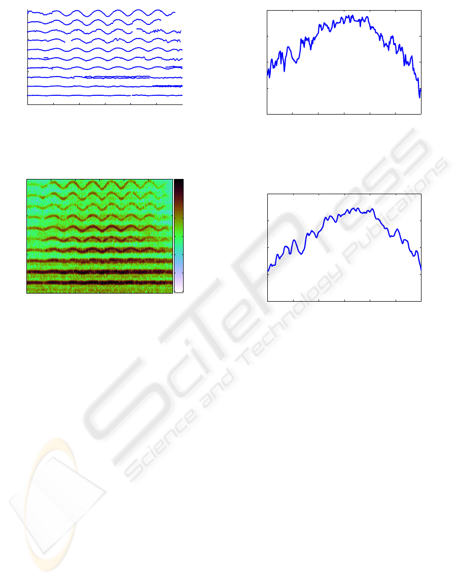
Figure 5: Frequency tracks obtained using the proposed
partial tracking algorithm. The signal under analysis is a
violin F8 tone played with vibrato.
Time (s)
Frequency (kHz)
0.2 0.4 0.6 0.8 1 1.2
0
5
10
−160
−140
−120
−100
−80
−60
−40
Figure 6: Spectrogram of the violin tone used in Example
2. The colorbar values are in dB.
4.4 Example 2: Results
The obtained partial tracks of the violin tone can
be seen in Figure 5. For comparison purposes the
spectrogram of the same tone is shown in Figure 6.
By comparing the spectrogram with the obtained
tracks, one can see that the frequency variations that
are characteristic of tone partials in vibrato playing
were well captured. Moreover, the tracks exhibited
a good smoothness with few discontinuities, being
those compatible with partial continuity failures also
visible in the spectrogram.
The amplitude variation of the 6th partial track
(centered around 8.3 kHz) can be viewed in Fig-
ure 7. Although being less well-behaved than the
frequency variation, the tracked amplitude variation
also exhibits coherent behavior. In order to confirm
that, the 6th partial has been isolated via an adequate
band-pass filtering of the tone. In the sequel, the per
frame energy of the selected partial was computed, as
seen in Figure 8. It can be observed that the evolu-
tion of the track amplitude over time closely matches
that of the selected partial energy, being their cross-
correlation coefficient equal to 0.95.
0.2 0.4 0.6 0.8 1 1.2
−80
−70
−60
−50
−40
Time (s)
Amplitude (dB)
Figure 7: Amplitude track obtained using the proposed par-
tial tracking algorithm. The plot shows in detail the sixth
partial of the violin tone.
0.2 0.4 0.6 0.8 1 1.2
−80
−70
−60
−50
−40
Time (s)
Amplitude (dB)
Figure 8: Overall energy variation of the 6th partial of the
violin tone.
5 CONCLUSIONS
This paper presented an adaptive lattice predictor to
the partial tracking problem in sinusoidal modeling
analysis of audio signals. The proposed method in-
corporated a novel predictor that significantly reduced
both the computational complexity as well as the
memory use in relation to previous methods. A new
heuristic to validate the predicted track parameters
was also described.
Simulations haveshownthat, under equivalenttest
conditions, the lattice predictor performs as effec-
tively as other methods previously reported in the lit-
erature, despite the reduced computational cost. In
order to confirm that, a real-world violin tone played
with vibrato has been subjected to analysis through
a sinusoidal modeling system that utilized the lattice
predictor within the partial tracking stage. The at-
tained results indicate that the adopted heuristics led
to a satisfactory tracking of the tone partials.
The proposed method may be further improved
if extended to perform partial tracking in a joint
SIGMAP 2008 - International Conference on Signal Processing and Multimedia Applications
90

frequency-amplitude prediction scheme. The deci-
sion algorithm could also be improved by considering
more than one frame, as proposed in (Lagrange et al.,
2007).
ACKNOWLEDGEMENTS
The authors wish to thank CNPq, CAPES, and
FAPERJ for supporting this work.
REFERENCES
Depalle, P., Garcia, G., and Rodet, X. (1993). Tracking
of partials for additive sound synthesis using hidden
markov models. In Proceedings of the 1993 IEEE In-
ternational Conference on Acoustics, Speech, and Sig-
nal Processing, volume 1, pages 225–228, Minneapo-
lis, USA.
Depalle, P. and H´elie, T. (1997). Extraction of spectral peak
parameters using a short-time fourier transform mod-
eling and no sidelobe windows. In 1997 IEEE Work-
shop Applications of Signal Processing to Audio and
Acoustics, New Paltz, USA.
George, E. B. and Smith, M. J. T. (1992). Analysis-by-
synthesis/overlap-add sinusoidal modeling applied to
the analysis and synthesis of musical tones. Journal
of the Audio Engineering Society, 40(6):497–516.
Laakso, T. and V¨alim¨aki, V. (1998). Energy-based effective
length of the impulse response of a recursive filter. In
Proceedings of the 1998 IEEE Conference on Acous-
tics, Speech, and Signal Processing, volume 3, pages
1253–1256, Seattle, USA.
Lagrange, M. and Marchand, S. (2007). Estimating the in-
stantaneous frequency of sinusoidal components using
phase-based methods. Journal of the Audio Engineer-
ing Society, 55(5):385 – 399.
Lagrange, M., Marchand, S., Raspaud, M., and Rault, J.-B.
(2003). Enhanced partial tracking using linear predic-
tion. In Proc. of the 6th International Conference on
Digital Audio Effects (DAFx’03), London, UK.
Lagrange, M., Marchand, S., and Rault, J.-B. (2007). En-
hancing the tracking of partials for the sinusoidal
modeling of polyphonic sounds. IEEE Transac-
tions on Audio, Speech, and Language Processing,
15(5):1625–1634.
McAulay, R. J. and Quatieri, T. F. (1986). Speech anal-
sysis/synthesis based on a sinusoidal representation.
IEEE Transactions on Acoustics, Speech, and Signal
Processing, 34(4):744–754.
Nunes, L., Esquef, P., and Biscainho, L. (2007a). Eval-
uation of threshold-based algorithms for detection
of spectral peaks in audio. In Proceedings of the
5th AES-Brazil Conference, pages 66–73, S˜ao Paulo,
Brazil.
Nunes, L., Merched, R., and Biscainho, L. (2007b). Re-
cursive least-squares estimation of the evolution of
partials in sinusoidal analysis. In Proceedings of the
2007 IEEE Conference on Acoustics, Speech, and Sig-
nal Processing, volume I, pages 253–256, Honolulu,
USA. IEEE.
Sayed, A. (2003). Fundamentals of Adaptive Filtering.
Wiley-IEEE.
Serra, X. (1997). Musical sound modeling with sinusoids
plus noise. In Poli, G. D., Picialli, A., Pope, S. T., and
Roads, C., editors, Musical Signal Processing. Swets
& Zeitlinger Publishers.
Serra, X. and Smith III, J. O. (1990). Spectral modeling
synthesis: A sound analysis/synthesis system based
on deterministic plus stochastic decomposition. Com-
puter Music Journal, 14(4):12–24.
Smith III, J. O. and Serra, X. (1987). PARSHL: An analy-
sis/synthesis program for non-harmonic sounds based
on a sinusoidal representation. In Proceedings of the
International Computer Music Conference, volume 76
(6), pages 1738–1742, Champaign-Urbana, USA.
Sterian, A. and Wakefield, G. H. (1998). A model-based
approach to partial tracking for musical transcription.
In Proceedings of the 1998 SPIE Annual Meeting, San
Diego, USA.
PARTIAL TRACKING IN SINUSOIDAL MODELING - An Adaptive Prediction-based RLS Lattice Solution
91
