IMPROVEMENT OF THE SIMPLIFIED FTF-TYPE ALGORITHM

Madjid Arezki, Ahmed Benallal, Abderezak Guessoum

LATSI Laboratory - Department of Electronics, Faculty of Engineering-University of Blida, Algeria

Daoud Berkani

Signal & Communications Laboratory - (ENP), Algiers, Algeria

Keywords: Fast RLS, NLMS, FNTF, Adaptive Filtering, Convergence Speed, Tracking capability.

Abstract: In this paper, we propose a new algorithm M-SMFTF which reduces the complexity of the simplified FTF-

type (SMFTF) algorithm by using a new recursive method to compute the likelihood variable. The

computational complexity was reduced from 7L to 6L, where L is the finite impulse response filter length.

Furthermore, this computational complexity can be significantly reduced to (2L+4P) when used with a

reduced P-size forward predictor. Finally, some simulation results are presented and our algorithm shows an

improvement in convergence over the normalized least mean square (NLMS).

1 INTRODUCTION

In general the problem of system identification

involves constructing an estimate of an unknown

system given only two signals, the input signal and a

reference signal. Typically the unknown system is

modelled linearly with a finite impulse response

(FIR), and adaptive filtering algorithms are

employed to iteratively converge upon an estimate

of the response. If the system is time-varying, then

the problem expands to include tracking the

unknown system as it changes over time (Haykin,

2002) and (Sayed, 2003). There are two major

classes of adaptive algorithms. One is the least mean

square (LMS) algorithm, which is based on a

stochastic gradient method (Macchi, 1995). Its

computational complexity is of O(L), L is the FIR

filter length. The other class of adaptive algorithm is

the recursive least-squares (RLS) algorithm which

minimizes a deterministic sum of squared errors

(Treichler, 2001). The RLS algorithm solves this

problem, but at the expense of increased

computational complexity of O(L

). A large number

of fast RLS (FRLS) algorithms have been developed

over the years, but, unfortunately, it seems that the

better a FRLS algorithm is in terms of computational

efficiency, the more severe is its problems related to

numerical stability (Treichler, 2001). The fast

transversal filter (FTF) (Cioffi, 1984) algorithm is

derived from the RLS by the introduction of forward

and backward predictors. Its computational

complexity is of O(L). Several numerical solutions

of stabilization, with stationary signals, are proposed

in the literature (Benallal, 1988), (Slock, 1991) and

(Arezki, 2007). Another way of reducing the

complexity of the fast RLS algorithm has been

proposed in (

Moustakides, 1999) and (Mavridis,

1996). When the input signal can be accurately

modelled by a predictor of order P, the fast Newton

transversal filter (FNTF) avoids running forward and

backward predictors of order L, which would be

required by a FRLS algorithm. The required

quantities are extrapolated from the predictors of

order P (P << L). Thus, the complexity of the FNTF

falls down to (2L+12P) multiplications instead of

8L. Recently, the simplified FTF-type (SMFTF)

algorithm (Benallal, 2007) developed for use in

acoustic echo cancellers. This algorithm derived

from the FTF algorithm where the adaptation gain is

obtained only from the forward prediction variables.

The computational complexity of the SMFTF

algorithm is 7L. In this paper, we propose more

complexity reduction of the simplified FTF-type

algorithm by using a new recursive method to

compute the likelihood variable. The computational

complexity of the proposed algorithm is 6L and this

computational complexity can be significantly

reduced to (2L+4P) when used with a reduced P-size

forward predictor. At the end, we present some

simulation results of the M-SMFTF algorithm.

156

Arezki M., Benallal A., Guessoum A. and Berkani D. (2008).

IMPROVEMENT OF THE SIMPLIFIED FTF-TYPE ALGORITHM.

In Proceedings of the International Conference on Signal Processing and Multimedia Applications, pages 156-161

DOI: 10.5220/0001940001560161

 SciTePress

2 ADAPTIVE ALGORITHMS

The main identification block diagram of a linear

system with finite impulse response (FIR) is

represented in

Figure 1.

Figure 1: Main block diagram of an adaptive filter.

The output a priori error

nL,

of this system at time

n is:

nnnL

−

(1)

where

nLnLn

−

= is the model filter output,

[]

121,

...,,,

+−−−

LnnnnL

xxxx is a vector containing

the last L samples of the input signal

x ,

[]

1,1,21,11,

...,,,

−−−−

nLnnnL

wwww is the coefficient

vector of the adaptive filter and L is the filter length.

The desired signal from the model is:

nLLoptnn

xw+=

(2)

where

[]

,2,1,

...,,,

Loptoptopt

Lopt

www=w represents

the unknown system impulse response vector and

v is a stationary, zero-mean, and independent noise

sequence that is uncorrelated with any other signal.

The superscript (.)

describes transposition. The

filter is updated at each instant by feedback of the

estimation error proportional to the adaptation gain,

denoted as

nL,

, and according to

nLnLnLnL ,,1,,

gww

−

(3)

The different algorithms are distinguished by the

gain calculation.

2.1 The NLMS Algorithm

The Algorithms derived from the gradient (Macchi,

1995), for which the optimization criterion

corresponds to a minimization of the mean-square

error. For the normalized LMS (NLMS) algorithm,

the adaptation gain is given by:

(4)

where

is referred to as the adaptation step and

is a small positive constant used to avoid division by

zero in absence of the input signal. The stability

condition of this algorithm is 0<

<2 and the fastest

convergence is obtained for

= 1 (Slock, 1993).

The power of input signal

nx,

is given by:

(5a)

It can alternatively be estimated using following

recursive equation (Gilloire, 1996):

1,,

)1(

nnxnx

γπγπ

+−=

−

(5b)

where

is a forgetting factor ( L/1≈

). The

computational complexity of the NLMS algorithm is

L multiplications per sample for the version with

the recursive estimator (5b).

2.2 The SFRLS Algorithm

The filter

nL,

w is calculated by minimizing the

weighted least squares criterion according to

(Haykin, 2002):

(

)

∑

−

−=

nLi

)( xww

(6)

where

λ denotes the exponential forgetting factor

<λ≤1). The adaptation gain is given by:



FRLS

RLS

nLnLnLnLnL

kxRg

−

(7)

where

nL,

R is an estimate of the correlation matrix

of the input signal vector. The variables

nL,

and

nL,

k respectively indicate the likelihood variable

and normalized Kalman gain vector. The calculation

complexity of a FRLS algorithm is 7

L. This

reduction of complexity has made all FRLS

algorithms numerically unstable. The numerical

stability is obtained by using some redundant

formulae of the FRLS algorithms (Benallal, 1988),

(Slock, 1991) and (Arezki, 2007). The numerical

stability is obtained by using a control variable,

called also a divergence indicator

(Arezki,

2007), theoretically equals to zero. Its introduction

in an unspecified point of the algorithm modifies its

numerical properties. This variable is given by:

⎩

⎨

⎧

≠

−=

practical0

theory0

(8)

where

,nL

r and

,nL

r are the backward a priori

prediction errors calculated differently in tree ways.

IMPROVEMENT OF THE SIMPLIFIED FTF-TYPE ALGORITHM

157

We define three backward a priori prediction errors

(

,nL

r ), theoretically equivalents, which

will be used to calculate the likelihood variable

nL,

the backward prediction error variance

nL,

and the

backward prediction

nL,

. We introduce these

variables into the algorithm, and we use suitably the

scalar parameters

),,(

μμμ

βγ

and

, in order to

obtain the numerical stability. For appropriate

choices, we selected the following control

parameters:

1,0 ===

μμμ

βγ

;

=0.5

(9)

It can be shown that the variance of the numerical

errors in the backward predictor, with the

assumption of a white Gaussian input signal, is

stable under the following condition (Arezki, 2007):

5.32

−=

(10)

These conditions can be written in another simpler

form

pL/11−=

, where the parameter p is a real

number strictly greater than 2 to ensure numerical

stability. The resulting stabilized FRLS (SFRLS)

algorithms have a complexity of 8L; it is given in

Table 1. Note that numerical stabilization of the

algorithm limits the range of the forgetting factor

(condition (10)) and consequently their

convergence speed and tracking ability.

Table 1: SFRLS (8L) algorithm.

Initialization:

100/

≥ ;

00,00,0,

;;1 EE

===

βλαγ

;

LLLLL

0,0,0,0,

==== kbaw

Variables available at the discrete-time index n:

1,1,1,1,1,1,1,

;;;;

;;

−−−−−−− nLnLnLnLnLnLnL

wkba

βαγ

New information:

x ,

Modeling of

x ,

−

1,, −−

−=

nLnLnnL

xe xa

;

⎥

⎦

⎤

⎢

⎣

⎡

−

⎥

⎦

⎤

⎢

⎣

⎡

⎥

⎦

⎤

⎢

⎣

⎡

−

λα

;

1,1,,1,,

−−−

nLnLnLnLnL

e kaa

;

,1,1,,

nLnLnLnL

−−

γλαα

;

nLnLLnnL

1,,

−−

−=

;

+−

nLnLnL

,11,

λβ

;

+−−

+−

nLnLnL

,11,1,

αγλ

])1[(

,, nLsnLsnLn

rrr

μμξ

+−−=

;

nnLnL

ξμ

γγ

;

nnLnL

ξμ

ββ

;

ξμ

;

1,,1,,

−

nLnLnLnL

k bkk

;

)(

−

λα

;

nLnL

nLnLnL

,,,1,,

kbb

−

;

,,1,,

)(

γλββ

nLnLnLnL

r+=

−

;

nLnLnnL

1,,

−

−=

;

nLnLnLnLnL ,,,1,,

kww

γε

−

2.3 The SMFTF Algorithm

The Simplified FTF-type (SMFTF) algorithm

(Benallal, 2007) derived from the FTF algorithm

where the adaptation gain is obtained only from the

forward prediction variables. The backward

prediction variables, which are the main source of

the numerical instability in the FRLS algorithms

(Benallal, 1988), (Slock, 1991) and (Arezki, 2007),

are completely discarded. By using only forward

prediction variables and adding a small

regularization constant

c and a leakage factor

we obtain a robust numerically stable adaptive

algorithm that shows the same performances as

FRLS algorithms.

Discarding the backward predictor does not

mean that the last components

nL,

are not updated,

but they are updated by components coming from

lower positions of

nL,

k . To avoid the instability of

the algorithm, we append a small positive constant

c to the denominator )/(

1,, anLnL

ce +

−

λα

, and it

might be preferable to have the forward predictor

nL,

return back to zero by doing

nL,

, where

is a close to one constant (Slock, 1993). The

computational complexity of the SMFTF algorithm

is 7L; it is given in Table 2.

Table 2: SMFTF (7L) algorithm.

Initialization:

LLLL

0,0,0,

=== kaw ; ;;1

00,0,

λαγ

== 100/

≥

Variables available at the discrete-time index n:

1,1,1,1,1,

;;;

;

−−−−− nLnLnLnLnL

wka

αγ

New information:

x ,

1,, −−

−=

nLnLnnL

xe xa

;

⎥

⎦

⎤

⎢

⎣

⎡

−

⎥

⎦

⎤

⎢

⎣

⎡

⎥

⎦

⎤

⎢

⎣

⎡

−

− 1,

anL

λα

;

{

}

1,1,,1,,

−−−

nLnLnLnLnL

e kaa

γη

;

,1,1,, nLnLnLnL

−−

γλαα

nLnL

xk+

;

nLnLnnL

1,,

−

−=

;

nLnLnLnLnL ,,,1,,

kww

γε

−

3 PROPOSED ALGORITHMS

3.1 The M-SMFTF Algorithm

We propose more complexity reduction of the

simplified FTF-type (M-SMFTF) algorithm by using

a new recursive method to compute the likelihood

variable. Let us replace the quantity (*), that has not

SIGMAP 2008 - International Conference on Signal Processing and Multimedia Applications

158

been used in

nL,

k of the MSFTF algorithm (Table

2), by the variable

, we obtain:

⎥

⎦

⎤

⎢

⎣

⎡

−

⎥

⎦

⎤

⎢

⎣

⎡

⎥

⎦

⎤

⎢

⎣

⎡

−

− 1,

anL

λα

(11)

By exploiting certain invariance properties by

shifting the vector input signal extended to the order

(L +1), we obtain two writing manners of input

vector:

[]

LnnL

−

= xx

(12a)

[]

−

nLn

x xx

(12b)

By multiplying on the left, the members of left and

right of the expression (11) by equations (12a) and

(12b) respectively, the following equality is

obtained:

−LnnLnLnL

anL

nLnL

−

−−

λα

(13)

By manipulating the relation (13), we obtain a new

recursive formula for calculating the likelihood

variable as given below:

1,,

−

nLnL

γδ

(14)

LnnL

anL

−

λα

(15)

After a propagation analysis of the numerical

errors of the 1

order and an asymptotic study of the

equations of errors propagation, we approximate the

errors in the forward variables (

nL,

aΔ ,

nL,

Δ ) and

the Kalman variables (

−

k ,

1, −

) by the

linear first order models deduced from

differentiating (

nL,

) and (

nL,

k ,

nL,

)

respectively. We can thus say that the system is

numerically stable, in the mean sense, for

and

between zero and one. It can be shown that the

variance of the numerical errors in the forward

predictor, with the assumption of a white Gaussian

input signal, is stable under the following condition:

)2(

)2(1

⎟

⎠

⎞

⎜

⎝

⎛

−++

−>

(16)

We notice that the lower bound of this condition

is always smaller than the lower bound of condition

(10) of the original numerically stable FRLS

algorithm, which means that we can choose smaller

values for the forgetting factor for the proposed

algorithm and consequently have faster convergence

rate and better tracking ability. The computational

complexity of the M-SMFTF algorithm is 6L; it is

given in Table 3.

Table 3: M-SMFTF (6L) algorithm.

Initialization:

LLLL

0,0,0,

=== kaw ; ;;1

00,0,

λαγ

== ; 100/

≥

Variables available at the discrete-time index n:

1,1,1,1,1,

;;;

;

−−−−− nLnLnLnLnL

wka

αγ

New information:

x ,

d .

1,, −−

−=

nLnLnnL

xe xa

;

⎥

⎦

⎤

⎢

⎣

⎡

−

⎥

⎦

⎤

⎢

⎣

⎡

⎥

⎦

⎤

⎢

⎣

⎡

−

− 1,

anL

λα

;

{

}

1,1,,1,,

−−−

nLnLnLnLnL

e kaa

γη

;

,1,1,, nLnLnLnL

−−

γλαα

LnnL

anL

−

λα

;

1,,

−

nLnL

γδ

nLnLnnL

1,,

−

−=

;

nLnLnLnLnL ,,,1,,

kww

γε

−

3.2 The Reduced M-SMFTF Algorithm

The Reduced size predictors in the FTF algorithms

have been successfully used in the FNTF algorithms

(

Moustakides, 1999), (Mavridis, 1996) and (Benallal,

2007). The proposed algorithm can be easily used

with reduced size prediction part. If we denote P the

order of the predictor and L the size of adaptive

filter, the normalized Kalman gain is given by:

⎥

⎦

⎤

⎢

⎣

⎡

−

⎥

⎦

⎤

⎢

⎣

⎡

⎥

⎦

⎤

⎢

⎣

⎡

−

anP

λα

(17)

where P is much smaller than L. The first (P+1)

components of the

nL,

k are updated using the

reduced size forward variables, the last components

are just a shifted version of the (P+1)

component of

nL,

k . For this algorithm, we need two likelihood

variables: the first one

nP,

, is used to update the

forward prediction error variance

nP,

, where

is (P+1)

component of

nL,

k . The second likelihood

variable

nL,

, is used to update the forward predictor

nP,

a of order P and the transversal filter

nL,

The computational complexity of this algorithm

is (2L+4P); it is given in Table 4.

IMPROVEMENT OF THE SIMPLIFIED FTF-TYPE ALGORITHM

159

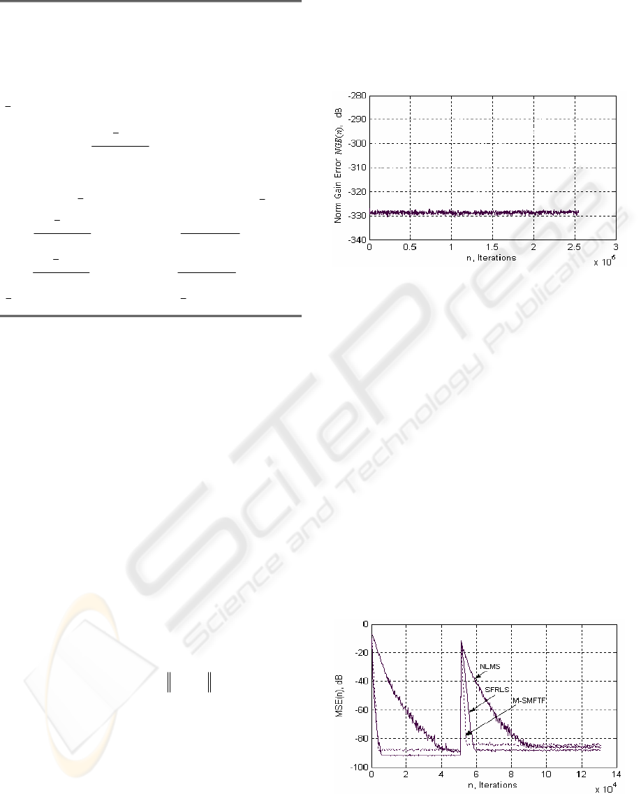
Table 4: Reduced M-SMFTF (2L+4P) algorithm.

Initialization:

100/

≥ ;

00,0,

;1 E

λαγ

== ;

;

LLL

0,0,

== kw ;

Variables available at the discrete-time index n:

1,1,1,1,1,

;;;

;

−−−−− nLnLnLnLnL

wka

αγ

;

New information:

1,, −−

−=

nPnPnnP

xe xa

;

⎥

⎦

⎤

⎢

⎣

⎡

−

⎥

⎦

⎤

⎢

⎣

⎡

⎥

⎦

⎤

⎢

⎣

⎡

−

anP

λα

;

):1(

1,1,

nLnP −−

= kk

;

)1(

+= Pc

nLnP

;

{

}

1,1,,1,,

−−−

nPnLnPnPnP

e kaa

γη

;

,1,1,, nPnPnPnP

−−

γλαα

PnnP

anP

−

λα

;

1,,

−

nPnP

γδ

;

LnnL

anP

−

λα

;

1,,

−

nLnL

γδ

;

nLnLnnL

1,,

−

−=

;

nLnLnLnLnL ,,,1,,

kww

γε

−

4 SIMULATION RESULTS

To confirm the validity of our analysis and

demonstrate the improved numerical performance,

some simulations are carried out. For the purpose of

smoothing the curves, error samples are averaged

over 256 points. The forgetting factor

and the

leakage factor

for the M-SMFTF algorithm are

chosen according to (16) with the stationary input. In

our experiments, we have used values of

comparable with the input signal power.

4.1 The M-SMFTF Case

We define the norm gain-error by )(nNGE . This

variable is used in our simulations to check the

equality of the expressions of the likelihood

variables. It is calculated by:

{

}

⎟

⎠

⎞

⎜

⎝

⎛

Δ=

,10

Elog10)(

nNGE g

(18)

where

(

)

nLnL ,

,,,

kkg

γγ

−=Δ is gain-error

vector,

nL,

and

nL,

are likelihood variables

calculated by SMFTF and M-SMFTF algorithms

respectively. We have simulated the algorithms to

verify their correctness. The input signal

x used in

our simulation is a white Gaussian noise, with mean

zero and variance one. The filter length is L=32, we

run the SMFTF and M-SMFTF algorithms with a

forgetting factor (

)/11( L

−

≥

)

=0.9688, the

leakage factor

=0.98 and

c =0.1. In Figure 2, we

give the evolution in decibels of the norm gain-

error

)(nNGE , we can see that the round-off error

signal stays constant. The M-SMFTF and the

SMFTF algorithms produce exactly the same

filtering error signal.

Figure 2: Evolution of the norm gain-error )(nNGE ;

L=32,

=0.9688,

=0.98,

c =0.1, E

=0.5.

We used a stationary correlated noise with a

spectrum equivalent to the average spectrum of

speech, called USASI noise in the field of acoustic

echo cancellation. This signal, with mean zero and

variance equal to 0.32, sampled at 16 kHz is filtered

by impulse response which represents a real impulse

response measured in a car and truncated to 256

samples. We compare the convergence speed and

tracking capacity of the M-SMFTF algorithm with

SFRLS and NLMS algorithms. The NLMS (

=1)

and SFRLS (

L3/11

−

) algorithms are tuned to

obtain fastest convergence. We simulated an abrupt

change in the impulse response by multiplying the

desired signal by 1.5 in the steady state at the

51200

samples. Figure 3 shows that better

performances in convergence speed are obtained for

the M-SMFTF algorithm.

Figure 3: Comparative performance of the M-SMFTF,

SFRLS and NLMS for USASI noise, L=256, M-SMFTF:

=0.9961,

=0.985,

c =0.5, E

=1; SFRLS:

=0.9987;

NLMS:

=1.

SIGMAP 2008 - International Conference on Signal Processing and Multimedia Applications

160

The differences in the final

)(nMSE for the M-

SMFTF and SFRLS algorithms are due to the use of

different forgetting factors

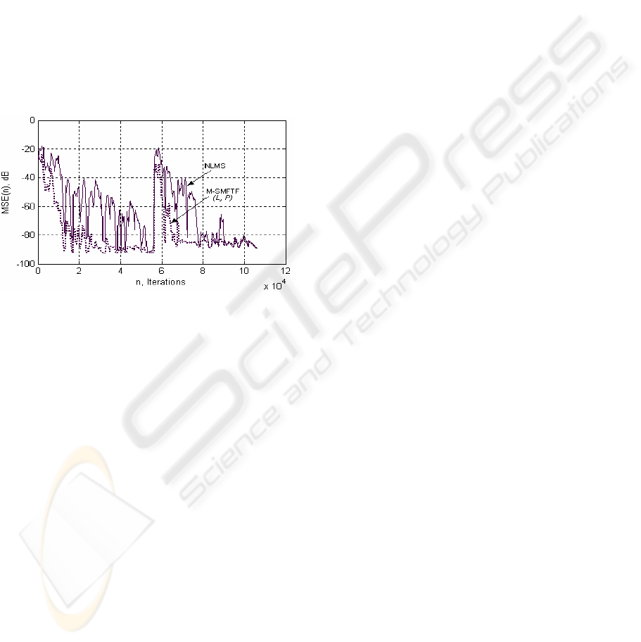
4.2 The Reduced M-SMFTF Case

In this simulation, we compare the convergence

performance of reduced size predictor M-SMFTF

algorithm and the NLMS algorithm. Figure 4

presents the results obtained with the speech signal,

sampled at 16 kHz, for the filter order L=256. We

simulated an abrupt change in the impulse response

at the 56320

samples. We use the following

parameters: the predictor order is P=20, the

forgetting factor is

P/11

−

. From this plot, we

observe that the re-convergence of M-SMFTF is

again faster than NLMS.

Figure 4: Comparative performance of the M-SMFTF and

NLMS with speech input, L=256, M-SMFTF: P=20,

=0.950,

=0.99,

c =0.1, E

=1; NLMS:

=1.

Different simulations have been done for

different sizes L and P, and all these results show

that there is no degradation in the final steady-

state

)(nMSE of the reduced size predictor algorithm

even for P<<L. The convergence speed and tracking

capability of the reduced size predictor algorithm

can be adjusted by changing the choice of the

parameters

and

c .

5 CONCLUSIONS

We have proposed more complexity reduction of

SMFTF (M-SMFTF) algorithm by using a new

recursive method to compute the likelihood variable.

The computational complexity of the M-SMFTF

algorithm is 6L operations per sample and this

computational complexity can be significantly

reduced to (2L+4P) when used with a reduced P-size

forward predictor (P<<L). The low computational

complexity of the M-SMFTF when dealing with

long filters and it a performance capabilities render

it very interesting for applications such as acoustic

echo cancellation. The simulation has shown that the

performances of M-SMFTF algorithm are better

than those of NLMS algorithm. The M-SMFTF

algorithm outperforms the classical adaptive

algorithms because of its convergence speed which

approaches that of the RLS algorithm and its

computational complexity which is slightly greater

than the one of the NLMS algorithm.

REFERENCES

Arezki, M., Benallal, A., Meyrueis, P., Guessoum A.,

Berkani, D., 2007. Error Propagation Analysis of Fast

Recursive Least Squares Algorithms. Proc. 9th

IASTED International Conference on Signal and

Image Processing, Honolulu, Hawaii, USA, August

20–22, pp.97-101.

Benallal, A., Gilloire, A., 1988. A New method to stabilize

fast RLS algorithms based on a first-order model of

the propagation of numerical errors. Proc. ICASSP,

New York, USA, pp.1365-1368

Benallal, A., Benkrid, A., 2007. A simplified FTF-type

algorithm for adaptive filtering. Signal processing,

vol.87, no.5, pp.904-917.

Cioffi, J., Kailath, T., 1984. Fast RLS Transversal Filters

for adaptive filtering. IEEE press. On ASSP, vol.32,

no.2, pp.304-337.

Gilloire, A., Moulines, E., Slock, D., Duhamel, P., 1996.

State of art in echo cancellation. In A.R. Figuers-vidal,

Digital Signal processing in telecommunication,

Springer, Berlin, pp.45–91

Haykin, S., 2002. Adaptive Filter Theory, Prentice-Hall.

NJ, 4

edition.

Macchi, O., 1995. The Least Mean Squares Approach with

Applications in Transmission, Wiley. New York.

Mavridis, P.P., Moustakides, G.V., 1996. Simplified

Newton-Type Adaptive Estimation Algorithms. IEEE

Trans. Signal Process, vol.44, no.8.

Moustakides, G.V., Theodoridis, S., 1999. Fast Newton

transversal filters - A new class of adaptive estimation

algorithms. IEEE Trans. Signal Process, vol.39, no.10,

pp.2184–2193.

Sayed, A.H., 2003. Fundamentals of Adaptive Filtering,

John Wiley & Sons. NJ,

Slock, D.T.M., Kailath, T., 1991. Numerically stable fast

transversal filters for recursive least squares adaptive

filtering,” IEEE transactions on signal processing,

vol.39, no.1, pp.92-114.

Slock, D.T.M., 1993. On the convergence behaviour of the

LMS and the NLMS algorithms. IEEE Trans. Signal

Processing, vol.42, pp.2811-2825.

Treichler, J.R., Johnson, C.R., Larimore, M.G., 2001.

Theory and Design of Adaptive Filter, Prentice Hall,

IMPROVEMENT OF THE SIMPLIFIED FTF-TYPE ALGORITHM

161