
ACCURATE AUTOMATIC SPOT ADDRESSING FOR MICROARRAY
IMAGES
M´onica G. Larese and Juan C. G´omez
Lab. for System Dynamics and Signal Processing, FCEIA, UNR
CIFASIS, CONICET, Bv. 27 de Febrero 210 Bis, Rosario, Argentina
Keywords:
Bioinformatics, cDNA microarrays, image analysis, automatic addressing.
Abstract:
In this paper a novel procedure based on texture spatial characterization techniques is proposed aimed at
automatically addressing spots in microarray images. The algorithm relies on the regular and pseudo-periodic
patterns of spots, which can be considered as texture primitives. A fully automatic procedure is proposed to
segment the autocorrelation functions of subgrid images and accurately determine the locations of the peaks.
These candidate peaks, i.e., vectors, are next used to compute the displacement vectors that fully characterize
the spatial arrangement of spots, describing the spot spacing and angle of rotation of the pattern. A refinement
procedure is then applied to improve the accuracy of the norms and angles of the displacement vectors. An
ideal template is generated using the computed spanning vectors, which is deformed and adjusted via Markov
Random Fields (MRF) modelling. Experiments based on artificial and real images are promising, showing
improvements regarding robustness against image rotations, and accuracy, over results provided by state-of-
the-art methods.
1 INTRODUCTION
A fundamental step in microarray image analysis is
the addressing of spots within image subgrids, in or-
der to measure the hybridization levels. Even though
spots are regularly located, this task is difficult due to
the low quality of the images. Current methods aimed
at addressing spots include semiautomatic (Heyer
et al., 2005; Yang et al., 2000; Eisen, 1999) and au-
tomatic (Ceccarelli and Antoniol, 2006; Hartelius and
Carstensen, 2003; Jain et al., 2002) procedures.
In this paper a new approach based on tech-
niques from texture spatial characterization is pro-
posed, where spots are considered as the texture prim-
itives. An autocorrelation segmentation procedure is
introduced in order to accurately estimate the two
displacement vectors which completely characterize
the lattice. After a refinement procedure, these vec-
tors define an ideal regular lattice which is finally de-
formed and adjusted using MRFs.
2 METHODOLOGY
2.1 Autocorrelation Segmentation
Autocorrelation was proposed for regular texture
structure characterization on general purpose images
in (Lin et al., 1997) and then applied with slight vari-
ations in (Liu et al., 2004). However, both procedures
lead to discrete displacement vectors, propagating the
errors to the estimated lattice of texture primitives.
In the present paper, a new approach is presented
to extract the spanning vectors using subpixel preci-
sion. In order to do this, the following operations are
applied on the autocorrelation image computed from
the microarray subgrid image:
1. Edge Detection via a LoG
1
filter and zero-
crossings detection (Gonzalez and Woods, 2002).
2. Morphological Reconstruction to fill holes in-
side object boundaries. After this step, two dif-
ferent cases may occur, viz., either separated or
non-separated connected components.
If the components are separated, skip step 3, oth-
erwise:
1
LoG: Laplacian of Gaussian
221
G. Larese M. and C. Gómez J. (2008).
ACCURATE AUTOMATIC SPOT ADDRESSING FOR MICROARRAY IMAGES.
In Proceedings of the International Conference on Signal Processing and Multimedia Applications, pages 221-224
DOI: 10.5220/0001941202210224
Copyright
c
SciTePress
3. Morphological Binary Opening trying circular
structuring elements with incremental radii, until
all the components are separated.
4. Connected Components Labelling.
5. Deletion of the components touching the border.
6. The Centroid Coordinates of each component
are regarded as the location of the candidate
peaks.
2.2 Displacement Vectors Calculation
The approach based on regions of dominance pro-
posed in (Liu et al., 2004) is applied to the centroids
computed in Section 2.1 in order to determine the
most prominent candidate peaks (regarded as vectors)
to be considered in the displacement vectors compu-
tation. Next, the procedure described in (Lin et al.,
1997), which is based on the generalized Hough trans-
form, is implemented in order to find the two vectors
that generate the spot lattice.
2.3 Spot Spacing and Angle of Rotation
Refinement
The norms of the two spanning vectors describe the
spot row and column spacings. Their angle describe
the deviation in each axis direction. In order to im-
prove accuracy even more, a histogram with the sizes
of the regions of dominance for all the candidate vec-
tors is constructed, as well as a histogram of the cor-
responding angles. The norms and angles of the two
displacement vectors computed in the previous Sec-
tion are used as entries to each one of these his-
tograms, and the weighted mean of the corresponding
isolated region in each histogram is regarded as the
corrected norm and angle for each spanning vector.
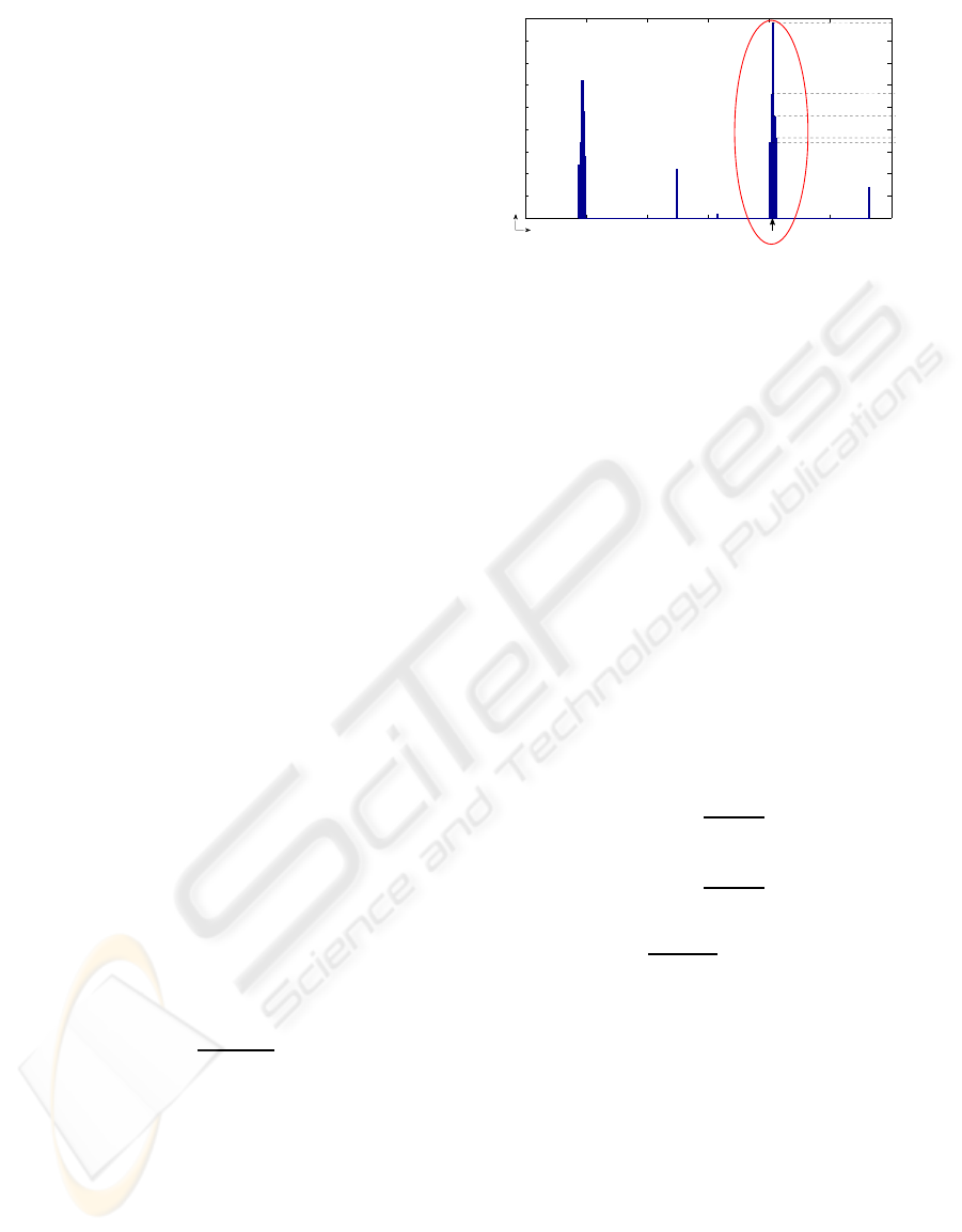
The procedure is illustrated in Fig. 1, where the
sizes of the regions of dominance (angles) histogram
is depicted. The corrected norm (angle) ∆
c
for each
one of the two spanning vectors is computed as
∆
c
=
∑
n
i=1
f
i
∆
i
n
∑
i=1
f
i
(1)
where f
i
and ∆
i
, i = 1, . . . , n stand for the frequencies,
and sizes of the regions of dominance (angles), re-
spectively. In the figure, ∆
′
represents the norm (an-
gle) computed in the previous Section for each one of
the displacement vectors (n = 5 in the example).
2.4 Template Adjustment via MRFs
A template grid can be constructed using the two pre-
viously estimated displacement vectors. The number
−2 −1.5 −1 −0.5 0 0.5 1
0
5
10
15
20
25
30
35
40
45
∆
i
f
i
f
1
f
2
f
3
f
4
f
5
∆
′
Figure 1: Illustration of the procedure for spots spacing and
angle of rotation refinement.
of rows, N
r
, and columns, N
c
, of spots are known a
priori from the microarrayer configuration. In order
to determine the starting position to span the template,
the top-leftmost spot of the real subgrid is determined
using the horizontal and vertical profiles of the tem-
porarily corrected for rotation image.
A first-order MRF (Geman and Geman, 1984) is
used to model the lattice of spots, allowing their lo-
cations to stochastically deviate from the ideal tem-
plate. The label set L = {l
i
= (x
i
, y
i
), i = 1, ..., N
r
N
c
}
contains the pairs of spatial coordinates for each node
site i, i.e., spot center, in the template.
The definition of an energy functional is heuris-
tic and application dependent, and theoretical ways of
determining it are not established yet (Amador J. J.,
2005). In this paper, the MRF functional to be mini-
mized was defined as
E
MRF
= E
lat
+ E
homog
(2)
E
lat
= α
0
∑
i∼ j
d
0
(i, j)
D
2
+
+ α
1
∑
i∼ j
d
1
(i, j)
D
− 1
2
− α
2
d
2
(i) (3)
E
homog
= β
µ(i)
σ(i) + 1
(4)
The term E
lat
controls the distortion of the grid. In
Eq. (3), d
0
(i, j) is the deviation in alignment between
neighboring nodes i and j, whereas d
1
(i, j) − D is the
deviation from the ideal fixed spot spacings D be-
tween i and j, as proposed by Carstensen (Carstensen
J. M., 1996).
On the other hand, d
2
(i) adopts one of two pos-
sible values: 0 or 1. In order to determine the d
2
(i)
value, the centroids of all the connected components
of the original microarray subgrid are computed. The
function d
2
(i) is then defined as follows
d
2
(i) =
(
1 if (x
i
, y
i
) coincides with a centroid
0 otherwise
(5)
SIGMAP 2008 - International Conference on Signal Processing and Multimedia Applications
222
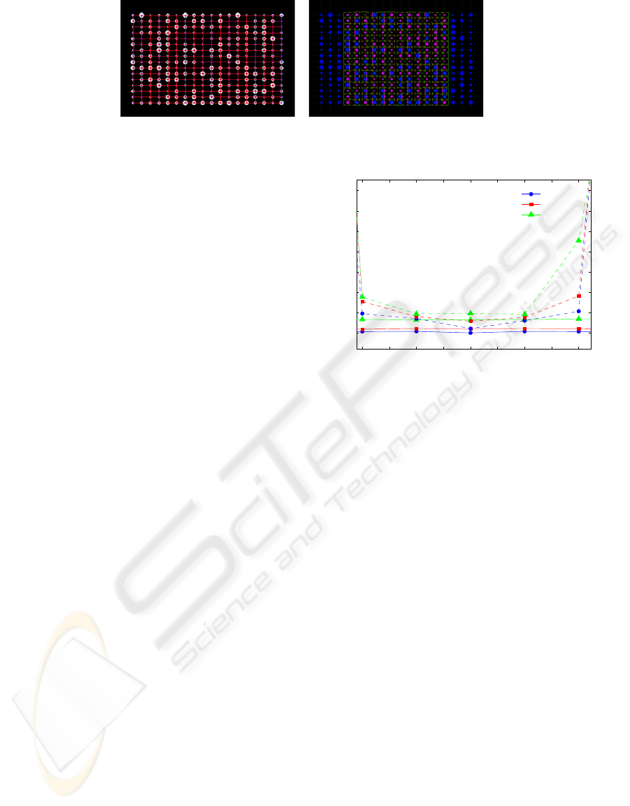
a. b.
Figure 2: Results of addressing a simulated image for the: a.) Proposed algorithm. b.) UCSF-Spot algorithm.
The term E
homog
measures the local intensity ho-
mogeneity around site i. For spot centers it is desir-
able to lie in homogeneous regions, such as the center
region of a spot. It is undesirable for them to lie on
borders. The local intensity mean value µ(i) and local
standard deviation σ(i) is computed on the 7x7 pixels
(not sites!) neighborhood of node site i.
The parameters α
0
, α1, α
2
and β are weights that
control the contribution of each term. In this work,
their values were experimentally set to 1, 10, 1000,
and 0.3, respectively. Minimization of the energy
functional was carried out using simulated annealing,
with an initial temperature of 0.8 and 1000 iterations.
3 EXPERIMENTAL RESULTS
In order to validate the proposed algorithm, experi-
ments on synthetic and real microarray images were
performed. Accuracy was assessed by means of
the RMSE (root-mean-square-error) between the es-
timated spot locations and the real ones.
3.1 Computer Generated Images
Two types of experiments were performed using syn-
thetic images. In the first case, subgrids with spot row
spacing different from column spacing, and random
spot sizes, were analyzed with the proposed method
and the UCSF-Spot automatic algorithm (Jain et al.,
2002). The results are shown in Figures 2(a) and (b),
respectively. As can be observed from Fig. 2(b) the
UCSF-Spot algorithm fails to address the spots, try-
ing to unify the row and column spacings. On the
other side, the proposed algorithm succeeds in locat-
ing the spots, as shown in Fig. 2(a), where the blue
crosses indicate the estimated spot centers.
In the second set of experiments, subgrids were
generated with equal row and column spacings, but
the locations of spots were randomly altered from
the regular lattice with Gaussian distributed variations
with zero mean and variances 0, 4 and 9. The images
were rotated with angles in the range [−5, 5] degrees
σ
2
= 0
σ
2
= 4
σ
2
= 9
Angle (in degrees)
Total RMSE (in pixels)
-2 -1
0
0
5
21
10
15
20
25
30
35
-1.5 -0.5 0.5 1.5
Figure 3: RMSE for the proposed and UCSF-Spot algo-
rithms (solid and dash-dotted lines, respectively) as a func-
tion of the image rotation angle.
and then analyzed with the proposed method and the
UCSF-Spot algorithm.
In Fig. 3 the RMSE for the proposed (solid line)
and UCSF-Spot (dash-dotted line) algorithms as a
function of the image rotation angle is depicted for
spot location variances equal to 0 (circles), 4 (squares)
and 9 (triangles). As it can be observed, the algo-
rithm introduced in this paper outperforms the UCSF-
Spot algorithm. In addition, it can be noticed that the
RMSE of the UCSF-Spot algorithm increases consid-
erably for rotation angles greater than 2 degrees, lead-
ing to unacceptable results.
In all the cases, the RMSE curve corresponding to
the proposed method is below 5 pixels, and below the
respective RMSE curves of UCSF-Spot.
3.2 Real Microarray Images
The proposed method was compared to the UCSF-
Spot algorithm and the accuracy of each method was
measured through the RMSE calculation on typical
real microarray images collected from the Standford
Microarray Database (SMD) (Demeter et al., 2007).
Details about the images, RMSEs in the x and y di-
rections and total RMSEs are reported in Table 1.
In all the cases under analysis, the proposed method
obtained a lower RMSE when compared to UCSF-
Spot. It is also worth noticing that (Ceccarelli and
ACCURATE AUTOMATIC SPOT ADDRESSING FOR MICROARRAY IMAGES
223

Table 1: Accuracy of spot addressing in terms of the RMSE (in pixels) for the proposed automatic algorithm and the UCSF-
Spot algorithm described in (Jain et al., 2002).
Image ID # spots
RMSE for the RMSE for
proposed method UCSF-Spot
RMSE
x
RMSE
y
Total RMSE RMSE
x
RMSE
y
Total RMSE
lc7b070rex2 (Alizadeh et al., 2000) 9216 1.56 1.52 2.18 44.21 4.97 44.49
lc7b017rex2 (Alizadeh et al., 2000) 9216 1.04 1.88 2.15 66.89 10.80 67.75
lc7b0104rex2 (Alizadeh et al., 2000) 9216 0.95 1.38 1.68 70.23 8.67 70.76
21028 (Subramanian et al., 2005) 43008 1.14 1.45 1.85 49.12 1.53 49.14
16275 (Subramanian et al., 2005) 45312 1.93 2.00 2.78 10.40 11.90 15.80
43957 (Subramanian et al., 2005) 43008 1.14 1.45 1.85 3.40 1.90 3.89
41602 (Subramanian et al., 2005) 43008 1.19 1.28 1.75 6.42 10.57 12.36
15739 (Arbeitman et al., 2002) 9216 1.76 1.66 2.42 7.67 6.45 10.02
Antoniol, 2006) also tested their method on images
21028, 16275, 43957, 41602 and 15739 reporting
higher RMSEs than the ones obtained by the method
proposed in this paper (image ID 51509 could not
be tested because it is no longer available for down-
load from SMD). The whole algorithm takes approx-
imately 15 seconds for a typical subgrid like this on a
1.6 GHz AMD-64 under Matlab and Linux, including
I/O operations.
4 CONCLUSIONS
In this paper an automatic approach is proposed to
address the location of microarray subgrid spot cen-
ters. The method relies on the assumption that spotted
microarray images can be regarded as regular texture
images and consequently texture spatial characteriza-
tion techniques are suitable to be applied. This is due
to the regularity and pseudo-periodicity exhibited by
microarray images.
Experimental results on synthetic and real images
show that the proposed method outperforms the ones
provided by a state-of-the-art microarray analysis tool
(namely the UCSF-Spot) especially when large im-
age rotations and unequal row and column spacings
are present. The present authors believe that the
method yields promising results improving accuracy
over widely used tools available in the literature.
REFERENCES
Alizadeh, A. A., Eisen, M. B. et al (2000). Distinct types
of diffuse large B-cell lymphoma identified by gene
expression profiling. Nature, 403(6769):503–511.
Amador J. J. (2005). Markov random field approach to re-
gion extraction using tabu search. J. Vis. Commun.
Image R., 16:134–158.
Arbeitman, M. N. et al (2002). Gene expression during
the life cycle of Drosophila melanogaster. Science,
297:2270–2275.
Carstensen J. M. (1996). An active lattice model in a
Bayesian framework. Comput. Vis. Image Und.,
63(2):380–387.
Ceccarelli, M. and Antoniol, G. (2006). A deformable
grid-matching approach for microarray images. IEEE
Trans. Image Proc., 15(10):3178–3188.
Demeter, J., Beauheim, C. et al (2007). The Stanford Mi-
croarray Database: implementation of new analysis
tools and open source release of software. Nucleic
Acids Res., 35(Database Issue):D766–770.
Eisen, M. (1999). Scanalyze. http://rana.lbl.gov/EisenSoft-
ware.html.
Geman, S. and Geman, D. (1984). Stochastic relaxation,
gibbs distributions and the bayesian restoration of im-
ages. IEEE Trans. P.A.M.I., 6:721–741.
Gonzalez, R. and Woods, R. (2002). Digital image process-
ing. Prentice Hall, 2nd. edition.
Hartelius, K. and Carstensen, J. M. (2003). Bayesian grid
matching. IEEE Trans. P.A.M.I., 25(2):162–173.
Heyer, L. J., Moskowitz, D. Z. et al (2005). Magic tool:
integrated microarray data analysis. Bioinformatics,
21(9):2114–2115.
Jain, A. N., Tokuyasu, T. A. et al (2002). Fully automatic
quantification of microarray image data. Genome Re-
search, 12:325–332.
Lin, H.-C., Wang, L.-L., and Yang, S.-N. (1997). Extracting
periodicity of a regular texture based on autocorrela-
tion functions. Pat. Recognition Letters, 18:433–443.
Liu, Y., Collins, R. T., and Tsin, Y. (2004). A computa-
tional model for periodic pattern perception based on
frieze and wallpaper groups. IEEE Trans. P.A.M.I.,
26(3):354–371.
Subramanian, S., West, R. B. et al (2005). The gene expres-
sion profile of extraskeletal myxoid chondrosarcoma.
J. Pathol., 206:433–444.
Yang, Y., Buckley, M. et al (2000). Comparison of
methods for image analysis on cDNA microarray
data. Tech. Report #584, Dep. of Stat., UCB. URL:
http://www.stat.berkeley.edu/users/terry/zarray/Tech-
Report/584.pdf.
SIGMAP 2008 - International Conference on Signal Processing and Multimedia Applications
224
