
IDENTIFICATION OF DISTRIBUTED PARAMETER SYSTEMS
BASED ON MULTIVARIABLE ESTIMATION AND
WIRELESS SENSOR NETWORKS
Constantin Volosencu
Automatics and Applied Informatics Department, “Politehnica” University of Timisoara
Bd. V. Parvan nr. 2, 300223 Timisoara, Romania
Keywords: System identification, distributed parameter systems, wireless sensor networks, multivariable estimation
techniques, auto-regression, heat distribution estimation.
Abstract: One of the important problem related to the usage of wireless sensor networks in harsh environments is the
identification of the states of the physical variables in the field, based on the measurements provided by the
sensors. The sensor networks allow the usage of the multivariable estimation techniques in distributed
parameter systems. The paper presents an application of a multivariable auto-regression estimation
technique for identification in distributed parameter systems, based on a sensor network. A case study was
presented for identification in a heat diffusion process.
1 INTRODUCTION
Sensor networks have proved their huge viability in
the real world in a variety of domains. Advances in
miniaturization, decreasing of their cost and power
and improvements in wireless networking and
micro-electro-mechanical systems have led to
research for large-scale deployment of wireless
sensor networks and formation of a new computing
domain. In the last years the deployment of small-
scale sensor networks in support of a growing array
of applications has become possible (Akyildiz,
2002), (Chong, 2003).
The distributed parameter systems are systems
whose state space is infinite dimensional. An object
whose state is heterogeneous has distributed
parameters. Partial differential equations are used to
formulate problems involving functions of several
variables, such as the propagation of sound or heat,
electrostatics, electrodynamics, fluid flow, elasticity
(Kubrusly, 1977).
Wireless sensor networks are extremely
distributed systems having a large number of
independent and interconnected sensor nodes, with
limited computational and communicative potential.
The sensor networks consist of hundreds or
thousands of heterogeneous disposable sensor nodes,
capable of sensing their environment and
communicating with each other via wireless
channels, coordinating and monitoring large areas.
Individually nodes possess properties such as
functionality and inter-node cooperation, under
limited energy reserves and technological
limitations. There are applications where the sensors
were generally bulky devices wired to a central
control unit whose role was to collect, process, and
act upon the data gathered by individual sensors. A
network of sensors could be developed with small
motion detectors, metal detectors, pressure detectors,
and vibration detectors, deployed around a valuable
asset.
The paper (Volosencu, 2008) presents a recent
survey of some characteristics of the sensor
networks, distributed parameters systems and
identification techniques, with examples of
applications of modeling of distributed systems in
sensor networks and identification based on
multivariable identification with auto-regression and
neural networks.
A strategy by which sensor nodes detect and
estimate non-localized phenomena such as
boundaries and edges (e.g., temperature gradients,
variations in illumination or contamination levels) is
study in (Novak, 2003).
92
Volosencu C. (2008).
IDENTIFICATION OF DISTRIBUTED PARAMETER SYSTEMS BASED ON MULTIVARIABLE ESTIMATION AND WIRELESS SENSOR NETWORKS.
In Proceedings of the International Conference on Wireless Information Networks and Systems, pages 92-95
DOI: 10.5220/0002026300920095
Copyright
c
SciTePress

2 PROPOSED METHOD
The following assumptions related to the sensor
network are made. The sensor network architecture
has a number of base stations deployed in the field.
Each base station forms a cell around itself that
covers part of the area. Mobile wireless nodes and
other appliances can communicate wirelessly. The
base station, acting as a controller and as a key
server, is assumed to be a laptop class device and
supplied with long-lasting power. Different sensor
network architectures may be used in practical
applications (Akyildiz, 2002), (Chong, 2003). For a
possible architecture some assumptions related to
the sensor nodes may be done. All the sensors are
similar in their computational and communication
capabilities and have enough memory to store up to
hundreds of bytes of data. The sensors may be static
and only the access points may be mobile. Each
sensor node knows its own location, even if they
were deployed by scattering or physical installation.
In a specific case the nodes can obtain their location
with location evaluation methods, after deployment
(Fig. 1).
Figure 1: Sensor network.
The information from different sensors is built
on the fact that actual sensor value is related with
past values provided by the same sensor. This
approach is based on a mathematical model that can
predict the value of one sensor by taking into
consideration the past and present values of
neighbouring sensors or of the implied sensor itself.
The computation implied in this approach is done at
the base station level. The proposed technique relies
on the fact that a sensor node is identified in the
moment that he starts to send data, using a linear
autoregressive multivariable predictor. The present
method considers that a multivariable autoregressive
(AR) model can efficiently approximate the time
evolution of the measured values provided by each
and every sensor within the coverage area. The AR
model definition is:
)()(...)1()(
1
tntxAtxAtx
n
ξ+−
+
+
−
=
(1)
where x(t) is a vector of the series under
investigation (in our case is the series of values
measured by the sensors from the network):
[
]
T
m
xxxx ...
21
=
(2)
and
i
A are the matrix of auto-regression coefficients,
n is the order of the auto-regression and
ξ
is a
vector containing the noise components that is
almost always assumed to be a Gaussian white
noise. By convention all the components
x
1
(t),…,x
n
(t) of the multivariable time series x(t) are
assumed to be zero mean. If not, another term (A
0
) is
added in the right member of equation (1). Based on
the model (1), (2) the coefficients A
i
may be
estimated in case that the time series x(t), x(t-
1),…,x(t-n) is known (recursive parameter
estimation), either predict future value
)t(x
^
in case
that A
i
coefficients and past values x(t-1),…, x(t-n)
are known (AR prediction). The method uses the
time series of measured data provided by each
sensor and relies on an autoregressive multivariable
predictor placed in base stations (Fig. 2).
Figure 2: Multivariable AR prediction.
The principle is the following: a sensor node will
be identified by comparing its output value
)t(x
with the value )t(x
ˆ
predicted using past/present
values provided by the same sensor. The proposed
methodology is described as follows. After this
initialisation, at every instant time t the estimated
value
)t(x
ˆ
A
is computed relying only on past values
x
A
(t-1), …, x
A
(0). First the parameter matrixes A
i
are
estimated using a recursive parameter estimation
method. There are a large number of methods for
obtaining AR coefficients (Ljung, 1999). An Armax
method, with zero coefficients for the inputs is used.
Second, the prediction value
)t(x
ˆ
is obtained using
the following equation:
)()(...)1()(
ˆ
1
tntxAtxAtx
AnAA
ξ+−
+
+
−
=
(3)
After that, the present value
)t(x
A
measured by
the sensor node may be compared with its estimated
value
)t(x
ˆ
A
by computing the error:
IDENTIFICATION OF DISTRIBUTED PARAMETER SYSTEMS BASED ON MULTIVARIABLE ESTIMATION
AND WIRELESS SENSOR NETWORKS
93
)(
ˆ
)()( txtxte
AAA
−=
(4)
If this error is higher than the threshold
A
ε
the
sensor A may be considered a potentially corrupted
sensor. There is no simple method to establish the
correct model order n in case of an AR model. Two
parameters can influence the decision: the type of
data measured by sensors and the computing
limitations. Because both of them are a priori
known, an off-line methodology is proposed.
Realistic values are between 3 and 6.
3 CASE STUDY
Let us consider a distributed parameter system,
described by a differential equation with partial
derivatives, for example the propagation of a
temperature wave in a homogenous planar field.
Several sensor nodes S
i,j,
i=1,…,N and j=1,…,M,
parts of a sensor network, are deployed in the
system. These sensors are measuring the local
variable (temperature θ [
o
C]). A regression model
that estimates the temperature value provided by the
sensor S
A
)t(
ˆ
)t(x
ˆ
AA
θ= by taking into
consideration the previous values of the data
provided by sensor x
A
(t-1), x
A
(t-2),…, x
A
(t-n) is
developed, with n chosen correlated to the above
consideration. The time distribution of the
temperature θ through the homogenous medium in
space is described by the equation:
),( tzθ=θ
(5)
where
)t,z(θ is the temperature at the moment t, at
distance z from the heat source. The heat conduction
is described by the heat equation (Ljung, 1994):
),(),(
2
2
tz
t
tz
z
c θ
∂
∂
=θ
∂
∂
θ
(6)
where c
θ
is the heat conductivity coefficient of the
medium. In order to investigate how the method
works, the function
),( tz
θ
=θ is sampled into the
aggregates
k,j
θ (temperature value provided by S
j,k
)
situated at the distance
k,j
z from the origin. The
energy conservation is governed for each point in
the field by the following equation:
kj
out
kj
inkj
PPW
dt
d
,,
,
−=
(7)
where
k,j
W is the energy stored in point (j,k),
kj
in
P
,
is the input power in the point and
kj
out
P
,
is the
output power from the point. The space model of the
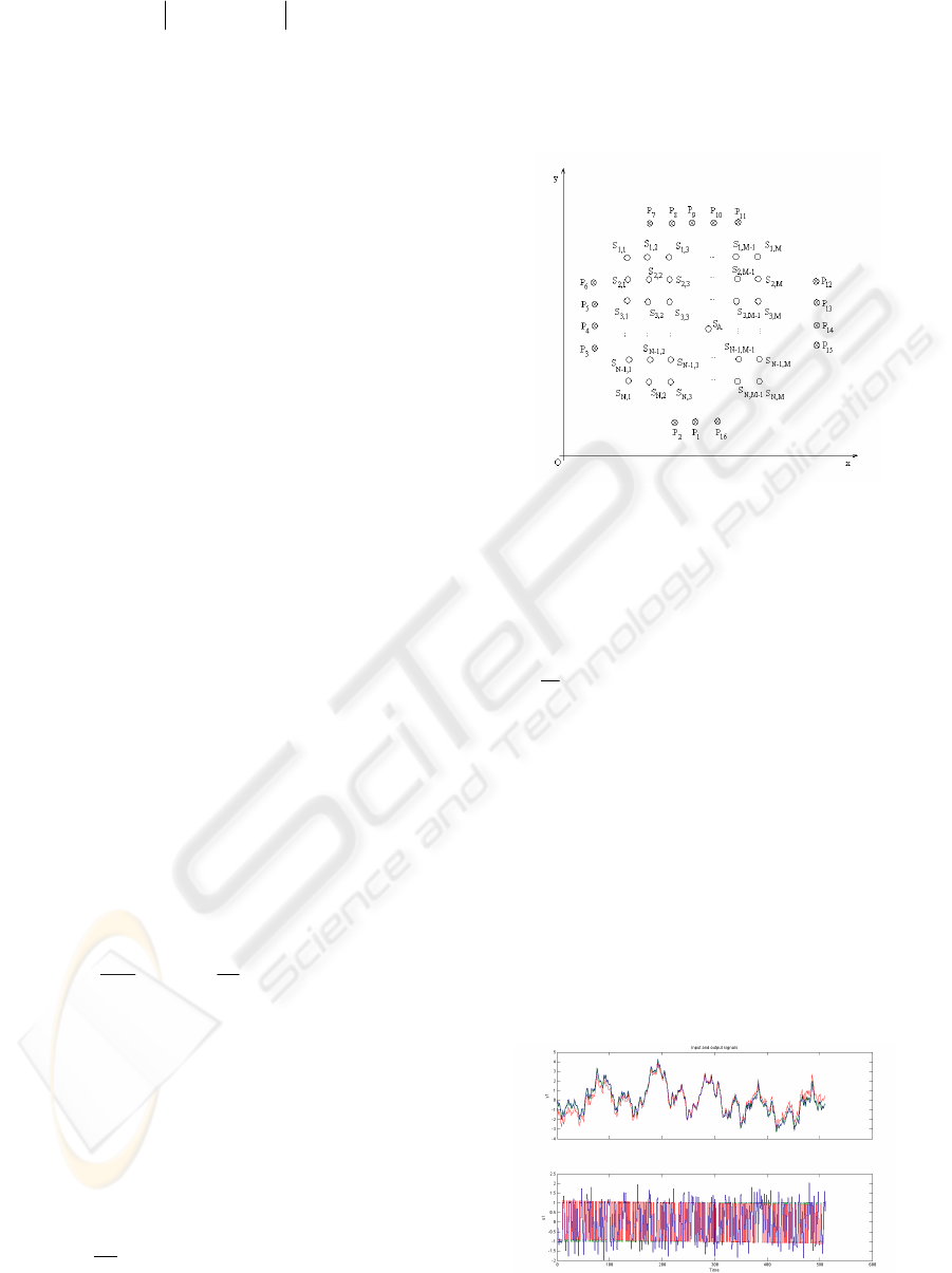
sensor deployed in the field with the heat sources is
presented in Fig. 3.
Figure 3: The deployment of the sensors.
Let the heat capacity of each point be denoted C
and the heat transfer coefficient between the points
kj
i
K
,
. These give the equation in time of the heat
diffusion:
∑
∑
θ−θ−
−θ−θ=θ
2
,,
2
,
2
1
,,
1
,
1
,
)]()([
)]()([)(
i
kjkj
i
kj
i
i
kjkj
i
kj
i
kj
ttK
ttKtC
dt
d
(8)
A discrete time equivalent equation of (8), with a
chosen adequate sample period h is used. Each cell
of sensors may receive inputs from the around
medium, from r sources with powers P
i
, i=1, …, r,
positioned around the network. The procedure is as
follows. 1. The input data for estimation was a
pseudo random binary signal for the powers P. The
output of the heat diffusion model x at these signals
was computed. Means and trends of the signals were
removed. The signals were filtered. The input P
1
and
the output x
1
in this case are presented in Fig. 4.
Figure 4: The input-output estimation data.
WINSYS 2008 - International Conference on Wireless Information Networks and Systems
94
2. A set with a multivariable model with 9 state
space equation for the cell and n=8 time delays for
the estimate was chosen. 3. The criterion of selected
the model was the residual from Fig. 5 and the fit of
the estimate in the simulation.
Figure 5: Residuals.
The multivariable estimation model with auto-
regression has 9x9x9=729 parameters which are
majority 0 and only on the diagonals of the 9
parameter matrix are nonzero values. For example,
the parameters of the estimation model for x
A
are
given in equation (9).
)(
)8(0112,0)7(022,0
)6(0286,0)5(019,0
)4(026,0)3(079,0
)2(302,0)(207,1)(
11
11
11
21
^
te
htxhtx
htxhtx
htxhtx
htxhtxtx
A
+
+−−−+
+−−−+
+−−−+
+−−−=
(9)
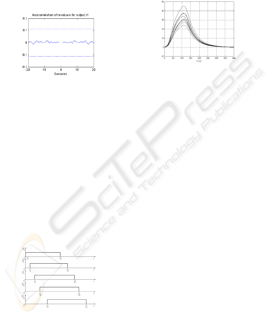
Four cases of travelling wave temperatures may
be taken in consideration, when four travelling
temperature waves pass on the North, South, West
and East sides of the cell, next to the sensor cell, as
it is presented in Fig. 2. For the North travelling
temperature wave the signal diagram of powers is
presented in Fig. 6.
Figure 6: A set of power test signals.
The response in temperature diffusion is
presented in Fig. 7. The estimation model may
generalize in the cases that the waves are passing
through diagonal face to the cell. When the error
e
A
(t) at the sensor S
A
passed over the threshold ε
A
,
imposed by the user, a decision must be taken.
Figure 7: The time response of the sensors, that fit the
estimate.
4 CONCLUSIONS
A multivariable method for identification of
distributed parameter systems based on sensor
networks is proposed based on an auto-regression
method with the values provide by the sensor
network. A case study was presented in a heat
diffusion process. An estimation model is developed
based on input-output data and residuals. The
estimation model was tested using travelling heat
waves. Being localized on a base station level, with
a reduced amount of computation the method is
suitable even for large-scale sensor networks.
REFERENCES
Akyildiz, I. F., Su, W., Sankarasubramaniam, Y., Cayirci,
E., 2002. Wireless Sensor Networks: A Survey. In
Computer Networks, 38(4).
Chong C.Y., Kumar, S. P., 2003. Sensor Networks:
Evolution, Opportunities, and Challenges. In
Proceedings of the IEEE, Vol. 91, No. 8.
Kubrusly, C.S., de S. Vincente, M. R., 1977. Distributed
parameter system identification. A survey, In
International Journal of Control, Vol. 26, Issue 4.
Ljung L., Glad, T., 1994. Modeling of Dynamic Systems,
Prentice Hall, Englewood Cliffs, NJ, 1994.
Nowak, R., Mitra, U., 2003. Boundary Estimation in
Sensor Networks: Theory and Methods. In
Proceedings of the First Int. Workshop on Information
Processing in Sensor Networks.
Volosencu, C., 2008. Identification in Sensor Networks, In
Proceedings of the 9
th
WSEAS Int. Conf. on
Automation and Information (ICAI’08), Bucharest.
IDENTIFICATION OF DISTRIBUTED PARAMETER SYSTEMS BASED ON MULTIVARIABLE ESTIMATION
AND WIRELESS SENSOR NETWORKS
95
