Descriptive Approach to Medical Image
Analysis - Substantiation and Interpretation
1
I. Gurevich,
1
V. Yashina,
2
H. Niemann and
3
O. Salvetti
1
Dorodnicyn Computing Center of the Russian Academy of Sciences, Vavilov str
Moscow, Russian Federation
2
University of Erlangen-Nuernberg, Lehrstuhl fuer Informatik, Martensstr
Erlangen, Germany
3
Institute of Information Science and Technologies, CNR, 1, Via G.Moruzzi
Piza, 56124, Italy
Abstract. The paper is devoted to the development and formal representation of
the descriptive model of information technology for automating morphologic
analysis of cytological specimens (lymphatic system tumors). The main
contributions are detailed description of algebraic constructions used for
creating of mathematical model of information technology and its specification
in the form of algorithmic scheme based on Descriptive Image Algebras. It is
specified the descriptive model of an image recognition task and the stage of an
image reduction to a recognizable from. The theoretical base of the model is the
Descriptive Approach to Image Analysis and its main mathematical tools. It is
demonstrated practical application of algebraic tools of the Descriptive
Approach to Image Analysis and presented an algorithmic scheme of a
technology implementing the apparatus of Descriptive Image Algebras.
1 Introduction
The paper is devoted to the development and formal representation of the descriptive
model of the information technology for automating morphologic analysis of
cytological specimens of patients with lymphatic system tumors. The main
contribution are detailed description of algebraic constructions used for creating of
mathematical model of the information technology and its specification in the form of
an algorithmic scheme based on Descriptive Image Algebras (DIA). We specify, in
particular, the descriptive model of an image recognition task and the stage of an
image reduction to a recognizable form.
The theoretical base of the model is the Descriptive Approach to Image Analysis
[1] and its main mathematical tools –DIA, Descriptive Image Models (DIM) and
Generating Descriptive Trees (GDT).
In a sense the results are continuation, specification and extension of the previous
research. In [3] we presented a brief introduction into the essential tools of the
Descriptive Approach (DIA, DIM, GDT), the simplified model of an image
recognition task based on multi-model image representation, a descriptive model of
Gurevich I., Yashina V., Niemann H. and Salvetti O. (2008).
Descriptive Approach to Medical Image Analysis - Substantiation and Interpretation.
In Image Mining Theory and Applications, pages 26-36
DOI: 10.5220/0002339900260036
Copyright
c
 SciTePress

the information technology, and the descriptive and the structural schemes of the
information technology. The state of the art and motivation were presented in our
previous publications [2, 3, 4].
Section 2 illustrates a simplified descriptive model of an image recognition task
based on multi-model image representation. In section 3 we introduce operands and
operations (and its operational (semantic) functions) of DIAs and Descriptive Image
Groups (DIG) necessary for constructing the algebraic model of the morphological
analysis of lymphatic cell nucleuses. Section 4 presents a descriptive model of the
information technology for automating morphologic analysis of cytological
specimens of patients with lymphatic system tumors. The technology has been tested
on the specimens from patients with aggressive lymphoid tumors and innocent tumor.
The results are discussed in Section 4.
The main components of the technology are described via DIA tools and presented
as an algorithmic scheme. The latter ensures a standard representation of technologies
for intellectual decision making.
2 Descriptive Model of an Image Recognition Problem
The Descriptive Approach provides the following model for an image recognition
process (Gurevich, 2005):
{}
{
}
rxnig
l
ysj
n
i
IPAMI )}({}{
...1
...1
...1
→→→
(1)
{
}
1...
i
n
I
- a set of initial images.
{}
1...
1
r
ig
n
I
K⊂∪
,
1...
{}
g
r
K
- a set of classes
determined by an image recognition task,
1...
{}
js
M - a multimodel representation of
each initial image
{
}
1...
i
n
I
. An algorithm combination
{
}
1...
y
l
A
solves an image
recognition problem, if it puts a set of predicates
{()}
g
irxn
PI
into correspondence to
the set of initial images, where predicate P
g
(I
i
)=a
ig
has the values: a
ig
=1, if an image I
i
belongs to a class K
g
; a
ig
=0, if an image I
i
does not belong to a class K
g
; a
ig
=∆, if an
algorithm combination does not establish membership of an image I
i
to a class K
g
.
Multi-model representation is generated by the set of GDT. Different ways for
constructing multi-aspect image representations may use different types of GDT. An
image representation becomes a multi-model one, if it is generated by different types
of GDT.
This model including a training stage is as follows:
{}
{
}
l
ys
j
a
n
i
pAMI
...1
2
...1
1
)(1
]
2
...[1
)(}{
1
⎯→⎯⎯⎯→⎯
{}
{
}
rxnig
l
ys
j
b
n
n
i
IPpAMI )}({)(}{
...1
0
3
...1
2
)(1
...1]
2
[
2
→⎯→⎯⎯⎯→⎯
+
(2)
The descriptive models could be represented as algorithmic schemes containing 3
stages: 1) an image reduction to a recognizable form (an image model (models)
construction); 2) training (adjusting parameters of chosen algorithms on a training set
of images); 3) recognition (sequential application of chosen algorithms with adjusted
2727

parameters to each image under recognition). Construction of a multi-model
representation is conceptually the same for both training set and recognition set;
however, as it will be shown below, training and recognition process can ramify in
stage 1. The latter consists of 2 sub-stages: 1(a) - construction of a multi-model
representation for training set; 1(b) construction of a multi-model representation for
recognition set. In accordance with chosen recognition algorithms the sub-stage 1(b)
is executed together with sub-stage 1(a) (a case of the same multi-model
representations for training and recognition sets), or it is executed after sub-stage 1(a)
(the sub-stage 1(a) defines multi-model representations for recognition set), or it is
executed after the stage 2. The latter is a case when recognition algorithm influences
the choice of multi-model representations for a recognition set.
3 Descriptive Image Algebras
In this section we introduce operands and operations (and its operational functions) of
DIAs and DIGs necessary for constructing the algebraic model of the morphological
analysis of lymphatic cell nucleuses.
DIA 1 is a set of color images. The operands: a set U of
{
}
I - a set of images
I={{(r(x,y), g(x,y), b(x,y)), r(x,y), g(x,y), b(x,y)
∈ [0...M-1]}, (x,y) ∈ X}, M=256 - the
value of maximal intensity of a color component, n - a number of initial images, X - a
set of pixels. The operations are algebraic operations of vector addition module M,
vector multiplication module M and taking an integral positive part of multiplication
module M by an element from the field of real numbers in each image point: 1)
I
1
+I
2
={{((r
1
(x,y)+r
2
(x,y)) mod M, (g
1
(x,y)+g
2
(x,y)) mod M, (b
1
(x,y)+b
2
(x,y)) mod M),
r
1
(x,y), r
2
(x,y), g
1
(x,y), g
2
(x,y), b
1
(x,y), b
2
(x,y) ∈ [0...M-1]}, (x,y) ∈ X}; 2)
I
1
·I
2
={{((r
1
(x,y)·r
2
(x,y)) mod M, (g
1
(x,y)·g
2
(x,y)) mod M, (b
1
(x,y)·b
2
(x,y)) mod M),
r
1
(x,y), r
2
(x,y), g
1
(x,y), g
2
(x,y), b
1
(x,y), b
2
(x,y) ∈ [0...M-1]}, (x,y) ∈ X}; 3)
αI={{([αr(x,y) mod M], [αg(x,y) mod M], [αb(x,y) mod M]), r(x,y), g(x,y), b(x,y)
∈
[0...M-1], α
∈ R}, (x,y) ∈ X}. DIA 1 is applied to describe initial images and the
multiplication operation of
DIA 1 is applied to describe segmentation of diagnostically
important nucleus on images.
DIG 1 is a set of operations sb((U,C)
→ U') for obtaining a binary mask corresponding
to an indicated lymphocyte cell nuclei, C - the information about the contours of
indicated nucleus, a set U' - a subset of a set U. If an image point (x,y) belongs to
indicated nuclei then r(x,y)=g(x,y)=b(x,y)=1, if a point (x,y) belongs to nuclei
background, r(x,y)=g(x,y)=b(x,y)=0. The operands: Elements of DIG 1 are
operations sb((U,C)
→ U') ∈ B. The operations of addition and multiplication are
introduced on the set of functions sb as sequential operations for obtaining a binary
masks and their addition and multiplication correspondingly: 1)
sb
1
(I,C)+sb
2
(I,C)=B
1
+B
2
; 2) sb
1
(I,C)·sb
2
(I,C)=B
1
·B
2
. DIG 1 is applied to describe a
segmentation process.
DIG 2 is a set U' of binary masks. The operands:
Elements of DIG2 are binary masks
B={{(r(x,y), g(x,y), b(x,y)), r(x,y), g(x,y), b(x,y)
∈ {0,1}, r(x,y)=g(x,y)=b(x,y)]}, (x,y)
∈ X}, M=256}. The operations of addition and multiplication are operations of union
2828

and intersection correspondingly: 1) B
1
+B
2
={{(r
1
(x,y) ∨ r
2
(x,y), g
1
(x,y) ∨ g
2
(x,y),
b
1
(x,y) ∨ b
2
(x,y)), r
1
(x,y), r
2
(x,y), g
1
(x,y), g
2
(x,y), b
1
(x,y), b
2
(x,y) ∈ {0,1}}, (x,y) ∈ X}; 2)
B
1
·B
2
={{(r
1
(x,y) ∧ r
2
(x,y), g
1
(x,y) ∧ g
2
(x,y), b
1
(x,y) ∧ b
2
(x,y)), r
1
(x,y), r
2
(x,y), g
1
(x,y),
g
2
(x,y), b
1
(x,y), b
2
(x,y) ∈ {0,1}}, (x,y) ∈ X}. DIG 2 is applied to describe binary masks.
DIA 2 is a set of gray scale images. The operands: A set V of {J} – a set of images J=
{{gray(x,y)}
(x,y) ∈ X
, (x,y) ∈ [0,...,M-1]}. The operations are algebraic operations of gray
functions addition module M, multiplication module M and taking an integral positive
part of multiplication module M by an element from the field of real numbers in each
image point: 1) J
1
+J
2
={{(gray
1
(x,y)+gray
2
(x,y)) mod M, gray
1
(x,y), gray
2
(x,y) ∈
[0..M-1]}, (x,y)
∈ X}; 2) J
1
·J
2
={{(gray
1
(x,y)·gray
2
(x,y)) mod M, gray
1
(x,y), gray
2
(x,y)
∈ [0..M-1]}, (x,y) ∈ X}; 3) αJ={{[α gray(x,y) mod M], gray(x,y) ∈ [0..M-1], α ∈ R},
(x,y)
∈ X}. DIA 2 is applied to describe separated nucleus on images.
DIA 3 – a set F of operations f(U
→ V) converting elements from a set of color images
into elements of a set of gray scale images. The operands: elements of DIA 3 -
operations f(U
→ V) ∈ F; such transforms can be used for elimination luminance and
color differences of images. The operations of addition, multiplication and
multiplication by an element from the field of real numbers are introduced on the set
of functions f as sequential operations of obtaining gray scale images and their
addition, multiplication and multiplication by an element from the field of real
numbers correspondingly: 1) f
1
(I)+f
2
(I)=J
1
+J
2
; 2) f
1
(I)·f
2
(I)=J
1
·J
2
; 3) αf(I)= αJ. DIA 3
is applied to eliminate luminance and color differences of images.
DIA 4 - a set G of operations g(V
→ P
1
) for calculation of a gray scale image features.
The operands: DIA 4 - a ring of functions g(V
→ P
1
) ∈ G, P
1
- a set of P-models
(parametric models). The operations. Operations of addition, multiplication and
multiplication by a field element are introduced on a set of functions g as operations
of sequential calculation of corresponding P-models and its addition, multiplication
and multiplication by a field element. 1) g
1
(J)+g
2
(J)=p
1
(J)+p
2
(J); 2)
g
1
(J)·g
2
(J)=p
1
(J)·p
2
(J); 3) αg(J)= αp(J). DIA 4 is applied to calculate feature values.
DIA 5 - a set P
1
of P-models. The operands: a set P
1
of P-models p=(f
1
, f
2
,…,f
n
), f
1,
,f
2
,…,f
n
- gray scale image features, n - a number of features. The operations: 1)
addition – an operation of unification of numerical image descriptions: p
1
+p
2
=(f
1
1
,
f
1
2
,…,f
1
n1
)+ (f
2
1
,f
2
2
,…,f
2
n2
)= (f
3
1
,f
3
2
,…,f
3
n3
), n
3
– a number of features of P-model p
1
plus a number of features of P-model p
2
minus a number of coincident features of P-
models p
1
; p
2
, {f
3
1
,f
3
2
,…,f
3
n3
} ⊂ { f
1
1
,f
1
2
,…,f
1
n1
, f
2
1
,f
2
2
,…,f
2
n2
} - different features and
coincident gray scale image features of P-models p
1
and p
2
; 2) multiplication of 2 P-
models – an operation of obtaining a complement of numerical image descriptions:
p
*
·p
2
=(f
1
1
,f
1
2
,…,f
1
n1
)*(f
2
1
,f
2
2
,…,f
2
n2
)=(f
4
1
,f
4
2
,…,f
4
n4
), n
4
- a number of significant
features of unified P-model of models p
1
and p
2
, f
4
1
,f
4
2
,…,f
4
n4
- significant features
obtained after analysis of features of P-model p
1
and P-model p
2
, f
4
1
, f
4
2
,…,f
4
n4
may
not belong to {f
1
1
, f
1
2
,…,f
1
n1
, f
2
1
,f
2
2
,…,f
2
n2
} and may consist from feature combinations;
3) multiplication by a field element - operation of multiplication of a number, a
vector, or a matrix by an element of the field: αp =α(f
1
, f
2
,…,f
n
)=(αf
1
, αf
2
,…, αf
n
). DIA
5
is applied to select informative features. The addition is applied for constructing
joint parametric image representation. The multiplication is applied for reducing a set
2929

of image features to a set of significant features. The multiplication by an element
from the field of real numbers is applied for feature vector normalization.
DIA 6 - a set P
2
of P-models (P
2
includes feature vectors of the same length). The
operands: a set P
2
of P-models p(J)=(f
1
(J),f
2
(J),…,f
n
(J)), n – a number of features,
f
1
(J),f
2
(J),…,f
n
(J) - gray scale image features, f
1
(J),f
2
(J),…,f
n
(J) ∈ R. The operations of
addition, multiplication and multiplication by a field element are introduced on the set
P
2
as operations of a vector addition, multiplication and multiplication by a field
element: 1) p(J
1
)+p(J
2
)=(f
1
(J
1
),f
2
(J
1
),…,f
n
(J
1
))+ (f
1
(J
2
),f
2
(J
2
),…,f
n
(J
2
))=(f
1
(J
1
)+f
1
(J
2
),
f
2
(J
1
)+f
2
(J
2
),…,f
n
(J
1
)+,f
n
(J
2
)); 2)
p(J
1
)*p(J
2
)=(f
1
(J
1
),f
2
(J
1
),…,f
n
(J
1
))*(f
1
(J
2
),f
2
(J
2
),…,f
n
(J
2
))=(f
1
(J
1
)·f
1
(J
2
), f
2
(J
1
)*
f
2
(J
2
),…,f
n
(J
1
)·,f
n
(J
2
)); 3) αp(J)=α(f
1
(J),f
2
(J),…,f
n
(J))=(α f
1
(J), α f
2
(J),…,α f
n
(J)). DIA 6
is applied to describe images reduced to a recognizable form.
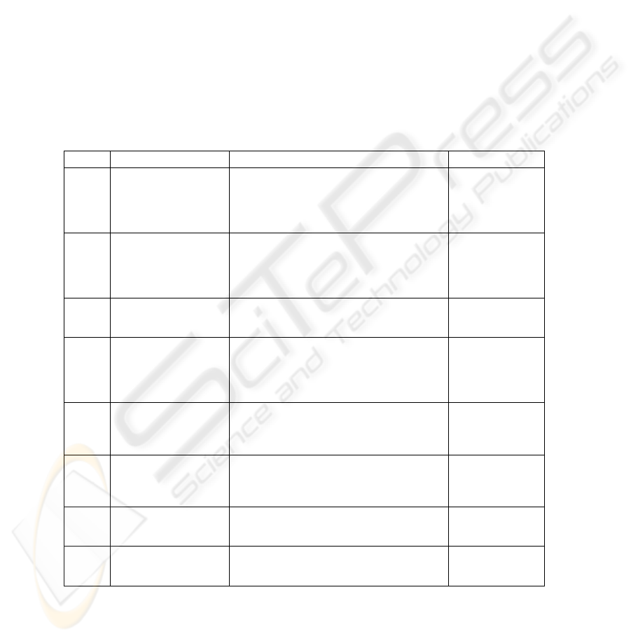
Table 1 shows all DIA with one ring and DIG used for describing the algorithmic
scheme for solving the task of cytological image recognition.
Table 1. DIAs with one ring used for describing algorithmic scheme for solving the task of
cytological image recognition.
Ring elements Ring operations Purpose
DIA1 color images
algebraic operations of vector addition
module M, vector multiplication module M
and taking an integral positive part of
multiplication module M by an element from
the field of real numbers in each image point
description of
initial images and
segmentation
process
DIG1
operations of
obtaining the binary
mask corresponds
indicated lymphocyte
cell nuclei
sequential operations for obtaining a binary
masks and their addition and multiplication
description of
segmentation
process
DIG2
binary masks
corresponds indicated
lymphocyte cell nuclei
algebraic operations of union and
intersection
description of
binary masks
DIA2 gray scale images
algebraic operations of gray functions
addition module M, multiplication module M
and taking an integral positive part of
multiplication module M by an element from
the field of real numbers in each image point
description of
separated nucleus
on images
DIA3
operations reducing
color images to gray
scale images
sequential operations of obtaining gray scale
images and their addition, multiplication and
multiplication by an element from the field
of real numbers
elimination
luminance and
color differences
of images
DIA4
operations of image
feature calculation
sequential calculation of corresponding P
(parametric)-models and its addition,
multiplication and multiplication by a field
element
feature
calculation
DIA5 P-models
image algebra operations (union,
complement, multiplication by real number)
selection of
informative
features
DIA6 P-models
operations of a vector addition,
multiplication and multiplication by a field
element
image reduction
to a recognizable
form
3030

4 An Algorithmic Scheme of the Morphological Analysis of the
Lymphoid Cell Nucleuses
The developed information technology will be described below and represented by
the algorithmic scheme (2) which is interpreted by means of DIA, DIM and GDT.
4.1 Initial Data
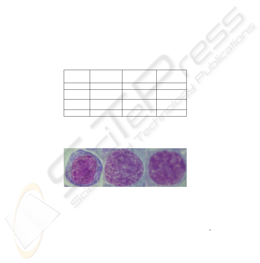
A database (DB) of specimens of lymphatic tissue imprints (Fig. 1) was created to
select and describe diagnostically important features of lymphocyte nuclei images.
DB contains 1830 specimens of 43 patients, both specimen images and the contours
of diagnostically important lymphocyte cell nucleus indicated by experts. The patients
belong to the following diagnostic groups: aggressive lymphoid tumors (de novo large
and mixed cell lymphomas (CL), transformed chronic lymphatic leukemia (TCLL)),
innocent tumor (indolent chronic lymphatic leukemia (CLL)).
Table 2. Database Statistics.
Diagnosis
Patient
number
Image number
Nuclei
number
CL
18 986 1639
TCLL
12 536 1025
CLL
13 308 2497
Total:
43 1830 5161
Footprints of lymphoid tissues were Romanovski-Giemsa stained and
photographed with digital camera mounted on Leica DMRB microscope using
PlanApo 100/1.3 objective (Fig. 1). The equivalent size of a pixel was 0,0036 mcm
2
.
24-bit color images were stored in TIFF-format.
Fig. 1. Specimen nucleus of patients with CL, TCLL and CLL diagnosis (from left to right).
4.2 Reducing an Image to a Recognizable Form
The initial images were divided into 2 groups: training image set
{
}
⎥
⎦
⎤
⎢
⎣
⎡
2
...1
n
i
I
and
recognition image set
{}
nn
i
I
...1]2/[ +
. The steps 1.1-1.6 of stage 1 “Reducing an image
to a recognizable form”) are described below as follows: description, step operands,
3131

step operations, results of step operation applying. It will be highlighted by letters ‘a’
and ‘b’ where processing of training and recognition sets differs.
Step 1.1. Obtaining Masks of Diagnostically Important Nucleus on Images.
Application of segmentation algorithm is described by operands sb((U,C)
→ U') ∈ B of
DIG1. An algorithm sb((U,C)
→ U') ∈ B is applied to initial images in order to obtain
corresponding mask (equation 3).
1
11
1
2
1
1
∈
⎯⎯⎯→
.
...
...
{}
{}
sb DIG
DIA
DIG
j
m
in
B
I
(3)
Step operands are initial images
{
}
n
i
I
...1
and contours of lymphocyte cell nucleus.
Step operation is an operation described by DIG1. Such description gives
flexibility for using different kind of segmentation algorithms. The applied algorithm
of threshold segmentation was supplemented by morphological processing of
derivable nuclei images in order to obtain a corresponding mask.
Results of operation applying are binary masks
1
j
m
B
...
{}
represented as operands
of DIG2.
Step 1.2. Segmentation of Diagnostically Important Nucleus on Images. The mask
multiplication by an initial image gives indicated nuclei image (equation 4).
11
1
12
1
2
11
11
•
≡⎯⎯⎯→
()
...
.
{}
... ...
( ) ...
{} ,{ }
{(,)}
DIA
j
m
DIA
DIA
T
I
in jm
ij j m
IB
MI B
(4)
Step operands are initial images
{
}
n
i
I
...1
and binary masks represented as
operands of DIG2.
Step operation is an operation of multiplication of 2 operands of DIA1. All initial
images were multiplied by corresponding binary masks.
The results of the operation are T(transfomatonal)-models
1
1...
{}
j
m
I of initial images.
Step 1.3. Reducing Color Images to Gray Scale Images. To compensate different
illumination conditions and different colors of stain the specimen images were
processed before feature values calculation (equation 5).
22
1
13
13
11
121
∈
≡⎯⎯⎯→
...
.
{}
... ...
{} { ()}
fDIA
j
m
DIA DIA
T
I
jm j m
IMI
(5)
Step operands are image models
1
1...
{}
j
m
I .
Step operations are described by the elements of the DIA 2. Such representation
gives flexibility for using different kinds of processing operations. Here the function
f(U→V)∈F (DIA 2 element) has a form (I={{(r(x,y),g(x,y),b(x,y)),r(x,y),g(x,y),b(x,y)
∈[0..M-1]}
(x,y) ∈X
}): f(I)=J={{gray(x,y)}
(x,y)∈X
, (x,y)∈[0...M-1]},
gray(x,y)=g(
x,y)
M
B2
, B - an average brightness of a blue component of an initial
RGB-image. The green tone in this case is the most informative.
The results of the operation are T-models
2
1...
{}
j
m
I .
Step 1.4a. Feature Calculation on Constructed Image Models of the Training Set.
To calculate different features the training set were processed by different operations
of DIA 4 (equation 6) (m
1
equals to a number of segmented nucleus in training set).
3232

12
1
4
11
14
35
22
111
11
∈
≡⎯⎯⎯⎯⎯→
{ , ,...}
...
.
{()}
... ...
{} { ()}
gg DIA
P
m
a
DIA DIA
P
Mj
jm j m
IMI
(6)
Step operands are image models
1
2
1...
{}
j
m
I .
Step operations are described by the elements of DIA 4. Such representation gives
flexibility for calculation of different features in order to obtain different P-models
1
P
Mj()
(elements of DIA 5). 47 features were selected for describing each of the
images: the size of nucleus in pixels, 4 statistical features calculated on the histogram
of nucleus intensity, 16 granulometric and 26 Fourier features of nucleus.
1
P
M
j
()
is
the vector with dimension 47 for each image model
2
j
I , j=1...m
1
.
The results of the operation are P-models
1
11...
{()}
P
m
Mj
.
Step 1.5a. Selection of Informative Features. This is an additional step of image
model reduction. As it will be shown below the recognition algorithm was applied to
both a full model
)(
1
jM
P
(j=m
1
+1...m) and a reduced model
)(
2
jM
P
(j=m
1
+1...m). At
this step the constructed descriptions of images from the training set are studied for
selecting the most informative features (equation 7).
1
5
21
15
56
11 21 1
11
+• •
≡⎯⎯⎯⎯→
(,, )
...
.
{()}
... ...
{()} {(())}
DIA P
m
a
DIA DIA
PPP
Mj
mm
Mj MMj
α
(7)
The step operands are image models
1
11...
{()}
P
m
Mj .
Step operations are described by the elements of DIA 5. Operations of addition
and multiplication are introduced for unificating and for reducing sets of image
features to a set of significant features. Operation of multiplication by an element
from the field of real numbers is introduced for normalization of feature vectors. Such
representation gives flexibility for using different kinds of feature analysis to obtain a
reduced set of features. Application of factor analysis to training image set detected
14 features with the largest loads in the first and second factor [4].
The results of the operation are P-models
1
21...
{()}
P
m
Mj - a the vector with
dimension 14 for each of image models
2
j
I , j=1...m
1
.
Step 1.6b. Feature Calculation on Constructed Image Models of the Recognition
Set. The steps 1.4 and 1.5 obtain a multi-model representation for training set. The
step 1.6 is the step of feature values calculation for a recognition set (equation 8).
12 4
11
16
6
3
22
121 1
1
2
1
1
∈
+
≡
+
⎯⎯⎯⎯⎯→
+
∨
( , , ...)
...
.
{()}
...
...
{() (())}{}
gg DIA
mm
b
DIA
DIA
PPP
j
jjmm
a
jm m
MI MMII
Ψ
(8)
Step operands are image models
1
2
1
+ ...
{}
j
mm
I .
Step operations are described by the elements of DIA 4. To describe each image
47 or 14 features were selected.
The results of the operation are P-models
11+ ...
{()}
mm
jΨ (note that the multi-model
representation of images was constructed).
3333

4.3 Training and Recognition
The class “Algorithms Based on Estimate Calculations” (AEC-class) were chosen as
recognition algorithms since they can be conveniently represented by algebraic tools
[5].
Initial Data. DIA 6 and its operands
22
121
PPP
jj
j
MI MMI() ( ) ( ( ))Ψ ≡∨ (j=1...m)
describe initial data for recognition algorithm
A (
12 n
j() ( , ,..., )
ψ
ψψ Ψ = - feature vector
with a dimension n=47 or n=14,
11mm
j
..
{()}Ψ
+
- information about recognition set,
1
1...
{()}
m
jΨ
- information about training set,
11
gj
rxm
gj
rxm
PI a{()} { }
′
=
- information about
memberships of training set images to classes
1...
{}
gr
K ( 01
gi
a {,}
∈
, r=3,
1
′
...
{}
j
m
I -
initial specimen images, one image for each indicated nucleus). Recognition
algorithm
11 1
111 1+−
=∈
.. ... ( ) ...
({ ( )} ,{ } ,{ ( )} ) { } { }
m
g
irxm m m
g
irxmm
y
l
Aj a j a AΨΨ
solves an image
recognition problem,
1...
{}
gj r
a - an information vector of image model
2
j
I calculated
by algorithm A (j=m
1
+1…m).
The algorithms were applied to both full image models
)(
1
jM
P
(j=1…m, 47
features) and reduced image models
)(
2
jM
P
(j=1…m, 14 features).
Algorithmic Scheme. We described the main steps and elements of an algebraic
model of information technology for automation of diagnostic analysis of cytological
specimens of patient with lymphatic system tumors (Fig. 2):
1
2
⎡⎤
⎢⎥
⎣⎦
...
{}
i
n
I
1
2
⎡⎤
+
⎢⎥
⎣⎦
...
{}
i
n
n
I
1...
{}
j
m
B
1
.
1
a
1
.
1
b
11...
{}
T
j
m
M
21..
{}
T
j
m
M
21..
{}
T
j
m
M
1
11..
{}
P
j
m
M
1
.
4
a
1
.
6
b
1
1+ ..
{}
j
mm
Ψ
1
21..
{}
P
j
m
M
1
{}
g
jrxm
Γ
o
p
1
−
′
()
{}
g
jrxmm
Γ
1.2 1.3
1.5
a
2.1
a
2.2
a
1
−()
{}
g
jrxmm
a
3.1
b
3.2
b
Fig. 2. Algorithmic scheme of information technology.
Discussion of the Results. The elements of the technology were tested via software
system «Recognition 1.0» [6] including AEC-algoritms. It appeared that the best
results are achieved by voting using all possible support sets, while automatic
selection of support set cardinality and selection of support sets of fixed cardinality
give lower precision.
Recognition rate for full feature set (Table 3) is 86,75%, while the rates differ for
different recognition classes. High recognition rate for CLL (97,84%) is probably
connected with innocent nature of CLL as opposed to CL (63,35%) and
TCLL(84,51%) - the malignant cases. Thus, cells of CLL have evident distinctions
from cells of other diagnoses, and cells of CL and TCLL are more similar to each
other.
3434

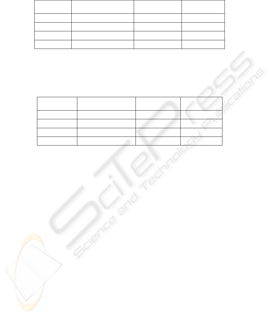
Table 3. The recognition rates for feature description consisted of 47 features.
Diagnosis
The number of correctly
recognized cells
Total number of
cells
The recognition
rate
CL 693 820 84,51%
TCLL 325 513 63,35%
CLL 1221 1248 97,84%
Total cell set 2239 2581 86,75%
The recognition rate reduced feature set (14 features) decreased to 83,18% (Table
4). This feature set includes following features: size of nucleus in pixels, average by
intensity histogram (statistic feature), numbers of elements with typical and minimal
size of nuclei (granulometric features), 9 Fourier-features of nucleus.
Table 4. The recognition rates using reduced feature description consisted of 14 features.
Diagnosis
The number of correctly
recognized cells
Total number of
cells
The recognition
rate
CL 626 820 76,34%
TCLL 300 513 58,48%
CLL 1221 1248 97,84%
Full cell set 2147 2581 83,18%
The software system «Recognition 1.0» [6] used for experimental investigation,
includes effective realization of AEC methods and allows to apply them for practical
task solution. It was experimentally verified that the best results are achieved by
voting using all possible support sets, while automatic definition of support set
capacity and definition of fixed support set capacity give lower precision.
5 Conclusions
The paper demonstrates practical application of algebraic tools of the Descriptive
Approach to Image Analysis - it is shown how to construct a model of a technology
for automation of diagnostic analysis on images using. It is presented an algorithmic
scheme of a technology implementing the apparatus of DIA.
The paper solves a dual task: it presents technology by well structured mathematic
model it shows how DIA can be used in image analysis application. The described
techniques and tools will be used for creating software implementation of the
technologies, its testing and performance evaluation.
Acknowledgements
This work was partially supported by the Russian Foundation for Basic Research
Grants Nos. 05-01-00784, 06-01-81009, 07-07-13545, by Collaborative project
3535

“Image Analysis and Synthesis: Theoretical Foundations and Prototypical
Applications in Medical Imaging” within agreement between CNR (Italy) and the
RAS, by the project “Descriptive Algebras with one ring over image models” of the
Program of Basic Research “Algebraic and Combinatorial Techniques of
Mathematical Cybernetics” of the Department of Mathematical Sciences of the RAS,
by the project no. 2.14 of the Program of the Presidium of the Russian Academy of
Sciences “Fundamental Problems of Computer Science and Information
Technologies”.
References
1. Gurevich, I.B., 2005. The Descriptive Approach to Image Analysis. Current State and
Prospects. In
Proceedings, 14
th
Scandinavian Conference on Image Analysis. LNCS 3540,
Springer-Verlag, Berlin Heidelberg.-P.214-223.
2.
Gurevich, I., Harazishvili, D., Jernova, I., et al, 2003. Information Technology for the
Morphological Analysis of the Lymphoid Cell Nuclei. In
Proceedings, The 13
th
Scandinavian Conference on Image Analysis
. LNCS 2749.-P.541-548.
3.
Gurevich, I., Koryabkina, I., Yashina, V., Niemann, H., and Salvetti, O., 2007. An
application of a Descriptive Image Algebra for Diagnostic Analysis of Cytological
Specimens. An Algebraic Model and Experimental Study. In
Proceedings, The 2th
International Conference on Computer Vision Theory and Applications, VISAPP 2007.
Volume Special Sessions, INSTICC Press.-P. 230-237
4.
Gurevich, I., Harazishvili, D.V. Salvetti, O., et al, 2006. Elements of Information
Technology for Cytological Specimen Image Analysis: Taxonomy and Factor Analysis. In
Pattern Recognition and Image Analysis: Advances in Mathematical Theory and
Applications
. Vol.16, No.1, Pleiades Publishing, Inc. 1. -P. 113-115
5.
Zhuravlev, Yu.I., 1998. An Algebraic Approach to Recognition and Classification
Problems. In
Pattern Recognition and Image Analysis: Advances in Mathematical Theory
and Applications, Vol.8.
MAIK "Nauka/Interperiodica".-P.59-100.
6.
Zhuravlev, Yu.I., Ryazanov, V.V., and others, 2005. RECOGNITION: A Universal
Software System for Recognition, Data Mining, and Forecasting. In
Pattern Recognition
and Image Analysis
, Vol. 15, No. 2. Pleiades Publishing, Inc.-P.476-478.
3636