Learning Probabilistic Models for Recognizing Faces

under Pose Variations

M. Saquib Sarfraz and Olaf Hellwich

Computer vision and Remote Sensing, Berlin university of Technology

Sekr. FR-3-1, Franklinstr. 28/29, Berlin, Germany

Abstract. Recognizing a face from a novel view point poses major challenges

for automatic face recognition. Recent methods address this problem by trying

to model the subject specific appearance change across pose. For this, however,

almost all of the existing methods require a perfect alignment between a gallery

and a probe image. In this paper we present a pose invariant face recognition

method centered on modeling joint appearance of gallery and probe images

across pose in a probabilistic framework. We propose novel extensions in this

direction by introducing to use a more robust feature description as opposed to

pixel-based appearances. Using such features we put forward to synthesize the

non-frontal views to frontal. Furthermore, using local kernel density estimation,

instead of commonly used normal density assumption, is suggested to derive

the prior models. Our method does not require any strict alignment between

gallery and probe images which makes it particularly attractive as compared to

the existing state of the art methods. Improved recognition across a wide range

of poses has been achieved using these extensions.

1 Introduction

Recent approaches to face recognition are able to achieve very low error rates in the

context of frontal faces. A more realistic and challenging task is to recognize a face at

a non-frontal view when only one (e.g. frontal) training image is available. Pose

variation in terms of pixel appearance, is highly non-linear in 2D, but linear in 3D.

Notable work such as [2] shows good results for recognition in the presence of pose

mismatch. A drawback of this, however, is the requirement of multiple gallery images

or depth information of the subject. From a practical stand point, we have at most a

single 2D gallery image per subject, and thus 2D appearance based methods have to

be further investigated for view independent recognition.

In the context of 2D appearance based methods, approaches addressing pose

variation can be categorized into two main bodies of work. Multi-view face

recognition is a direct extension of frontal face recognition in which the algorithms

require gallery images of every subject at every pose [1]. In this context, to handle the

problem of one training example, recent research direction has been to use specialized

synthesis techniques to generate a given face at all other views and then perform

conventional multi-view recognition[7][4]. Such synthesis techniques, however,

suffers from severe artifacts and are not sufficient to preserve the identity of a person

in general.

Saquib Sarfraz M. and Hellwich O. (2008).

Learning Probabilistic Models for Recognizing Faces under Pose Variations.

In Image Mining Theory and Applications, pages 122-132

DOI: 10.5220/0002341001220132

 SciTePress

The other very recent line of work has been to directly model the local appearance

change, due to pose, across same subjects and among different subjects. Differences

exist among different methods, in how these models are built, but the goal of all is

same i.e. trying to approximate the joint probability of a gallery and probe face across

different pose [5][11][17]. Such an approach is particularly attractive in that it does

not depend on error prone synthesis and it also automatically solves the one training

image problem in a principled way as these appearance models can be learned

effectively from an offline database of representative faces. Another benefit of such a

line of work is that adding a new person’s image in the database does not require

training the models again. We note, however, almost all of these methods proposed in

literature until now intrinsically assume a perfect alignment between a gallery and

probe face in each pose. This alignment is needed, because, otherwise, in current

appearance-based methods it is not possible to discern between the change of

appearance due to pose and change of appearance due to the local movement of facial

parts across pose.

In this contribution, we introduce novel extensions in this line of work and propose

to build models on features which are robust against misalignments and thus do not

require the facial landmarks to be detected as such. Our approach, briefly, is to learn

probabilistic models describing the approximated joint probability distribution of a

gallery and probe image at different poses. Since we address the problem where at

most one training image (e.g. frontal) is available, we learn such models by explicitly

modeling facial appearance change between frontal and other views when identity of

a person is same and when it is different across pose. This is done by computing

similarities between extracted features of faces at frontal and all other views. The

distribution of these similarities is then used to obtain the likelihood functions of the

form.

(I ,I |C ), C {S,D}∈

(1)

‘C’ refers to classes where the gallery ‘I

’

and probe ‘I

’

images are similar (S) and

dissimilar (D) in terms of subject identity. For this purpose an independent generic set

of faces, at views we want to model, is used for offline training.

A contribution is made in this paper towards improved recognition performance

across pose without the need of properly aligning gallery and probe images. To

achieve this, we propose to use an extension of SIFT features [12], that are

specifically adapted for the purpose of face recognition in this work. This feature

description captures the whole appearance of a face in a rotation and scale invariant

manner, and is shown robust with regards to variation of facial appearance due to

localization problems [14]. Furthermore, we propose to synthesize these features at

non-frontal views to frontal by using multivariate regression techniques. The benefit

of this in recognition performance is demonstrated empirically. To approximate the

likelihood functions in equation 1, we propose to use local kernel density estimation

for deriving models as opposed to commonly used Gaussian Model.

123123

2 Modeling whole Face Appearance Change across Pose

Our approach is to extract whole appearance of the face in a manner which is robust

against misalignment due to localization. For this we use feature description [12] that

is slightly adapted for the purpose of face recognition in this work. It models the local

parts of the face and combines them into a global description. We then synthesize

features at non-frontal views to frontal. Computing similarities using these features

between frontal and other poses provides us with prior distribution for each pose.

These distributions are then modeled using a variant of local kernel density estimator

instead of commonly assumed Gaussian model.

We show, in section 2.4, that deriving model using local kernel density results in a

better fit than assumed Gaussian model. The effectiveness of our method is

demonstrated using CMU Pose, Illumination and Expression (PIE) database [15].

2.1 Facial Database

We use CMU PIE database for training and testing of our models. The PIE database

consists of 68 subjects imaged under 13 poses, 21 illumination conditions and 3

expression variations. We use the pose portion of this database with frontal

illumination and neutral expression in all 13 poses. Each pose is approximately 22.5

apart.

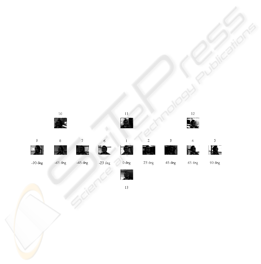
As depicted in figure 1, the pose varies from pose 1(frontal) to pose 9(left-

profile) with pose 5(Right-profile). Where pose 10, 11, 12 and 13 correspond to up

and down tilt of the face in corresponding poses.

Fig. 1. 13 poses covering left profile (9), frontal (1) to right profile(5), and slightly up/down tilt

in pose 10, 11, 13 and 12 of corresponding poses in 8, 1 and 4 respectively.

Images of half of the subjects are used as offline training set for training of models,

while other half are used for testing. Face windows are cropped from the database

without employing any commonly used normalization procedure. Therefore images

contain typical variations that may arise due to miss-localization like scale, part

clippings and background. All images are then resized to 128x128 pixels.

Typical variations present in the database are depicted in few of the example

images in figure 2.

124124

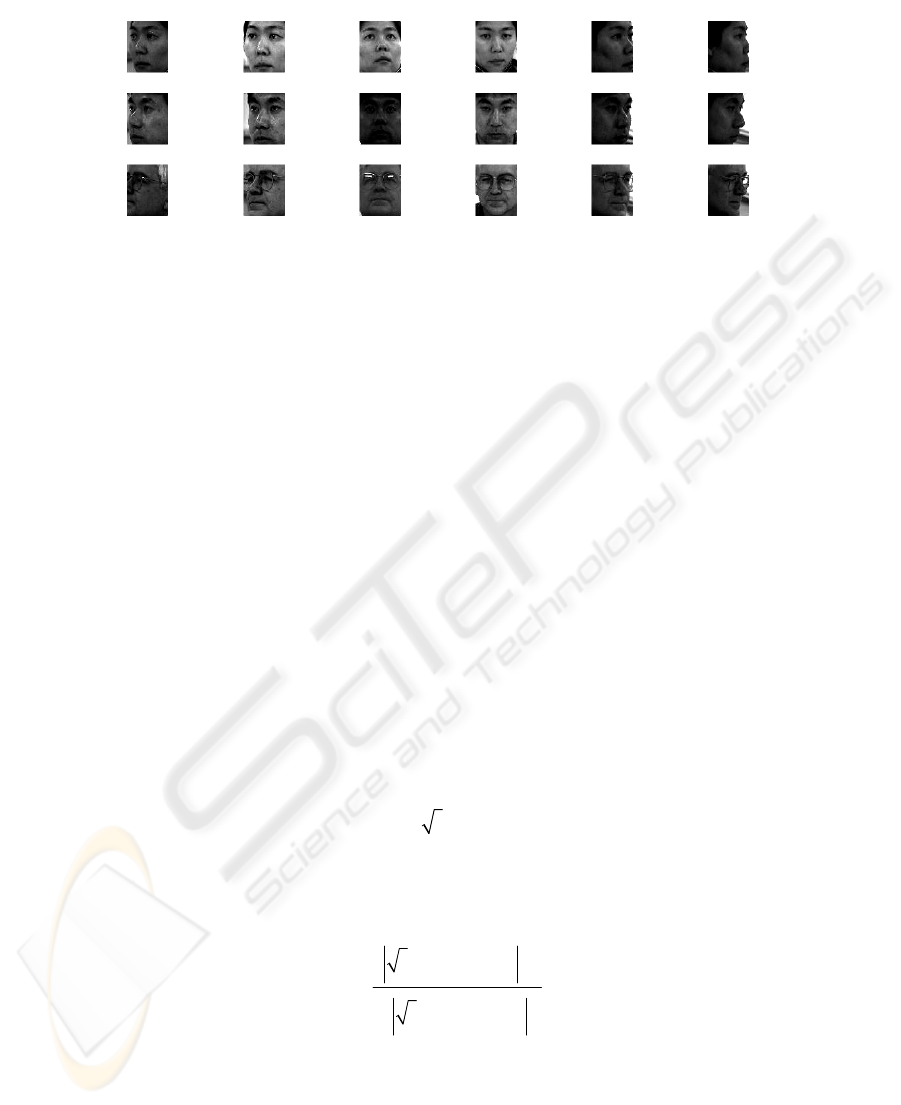
Fig. 2. Examples of cropped facial images depicting typical variations due to miss-localization

e.g. scale, part clipping, background etc.

Note that, since we do not employ any kind of normalization such as fixing eye

location or eye-distance, face images across pose suffer from typical misalignment.

2.2 Feature Extraction

As described earlier, commonly used facial representations are related directly to

pixel intensities and, as such, are not invariant to changes in scale, position,

orientation, brightness and contrast of a face. Since these types of transformations are

to be expected after a face detector stage, alignment by using several facial landmarks

is needed.

We propose to use a representation based on gradient location-orientation

histogram (GLOH) [12], which is more sophisticated and is specifically designed to

reduce in-class variance by providing some degree of invariance to the

aforementioned transformations. GLOH features are an extension to the descriptors

used in the scale invariant feature transform (SIFT) [9], and have been reported to

outperform other types of descriptors in object recognition tasks [12].

The extraction procedure has been slightly adapted to the task of face recognition

and will be described in the remainder of this section.

The extraction process begins with the computation of scale adaptive spatial

gradients for a given image I(x,y). These gradients are given by

w(x, y,t) t L(x, y;t)

∇≡ ∇

∑

(5)

where L(x,y; t) denotes the linear Gaussian scale space of I(x,y) [8] and w(x,y,t) is a

weighting, as given in equation 6.

tL(x,y;t)

w(x, y,t)

tL(x,y;t)

∇

∑

(6)

125125

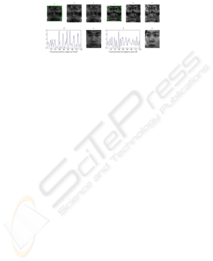
Fig. 3. (a-b) Gradient magnitudes (c) polar-grid partitions (d) 128-dimentional feature vector

(e). Example image.

The gradient magnitudes obtained for two example images (figure 3. e) are shown

in figure 3.b. The gradient image is then partitioned on a grid in polar coordinates, as

illustrated in figure 3.c. The partitions include a central region and seven radial

sectors. The radius of the central region is chosen to make the areas of all partitions

equal. Each partition is then processed to yield a histogram of gradient magnitude

over gradient orientations. The histogram for each partition has 16 bins corresponding

to orientations between 0 and 2π, and all histograms are concatenated to give the final

128 dimensional feature vector, see figure 3.d.

It should be noted that, in practice, the quality of the descriptor improves when

care is taken to minimize aliasing artifacts. The recommended measures include the

use of smooth partition boundaries as well as a soft assignment of gradient vectors to

orientation histogram bins.

2.3 Synthesizing Features at Non-Frontal Views to Frontal

It is well known that when a large number of subjects are considered, the recognition

performance of appearance-based methods deteriorates significantly. It is due to the

fact that distribution of face patterns is no longer convex as assumed by linear models.

By transforming the image in the previous section into a scale and rotation invariant

manner, we assume that there exists a certain relation between these features of

frontal and posed image that we can linearly transform. We justify this assumption by

comparing the similarity distributions estimated from non-synthesized GLOH features

and synthesized features. One simple and powerful way of relating these features is to

use the regression techniques. Let us suppose that we have the following multivariate

linear regression model, for finding relation between the feature vectors of frontal ‘I

’

and

any other angle I

= I

(7)

ββ

p1 (1,1) (1,D)

ββ

II1

(D+1,1) (D+1,1)

⎡⎤⎡ ⎤

⎡

⎤

⎢⎥⎢ ⎥

⎢

⎥

⎢⎥⎢ ⎥

⎢

⎥

⎢⎥⎢ ⎥

⎢

⎥

⎢⎥⎢ ⎥

⎣

⎦

⎣⎦⎣ ⎦

MM MOM

(8)

126126

Where n > D+1, with D being the dimensionality of each

and

. B is a pose

transformation matrix of unknown regression parameters, under the sum-of-least-

squares regression criterion, B can be found using Moor-Penrose inverse.

T-1T

PP PF

B=(I I ) I I

(9)

This transformation matrix B is found for each of the poses Ip (±22.5

, ±45, ±65

±90

) with frontal 0

‘I

’.

Given a set of a priori feature vectors (from an offline training set

), representing

faces at frontal ‘I

’ and other poses ‘I

’, we can thus find the relation between them.

Any incoming probe feature vector can now be transformed to its frontal counterpart

using: I

· B

2.4 Obtaining Prior Pose Models for Recognition

We approximate the joint likelihood of a probe and gallery face as:

gp pg gp

(I ,I |C,Ø ,Ø ) p( |C,Ø ,Ø )

≅

(10)

Where ‘C’ refers to classes where the gallery ‘I

’

and probe ‘I

’

images are similar (S)

and dissimilar (D) in terms of subject identity. ‘

’ is the similarity between gallery

and probe image. Cosine measure is used as a similarity metric. These likelihoods for

the similar and dissimilar class are then found by modeling the distribution of

similarities of extracted features between frontal and every pose from offline training

set.

Figure 4 depicts the histograms for the prior same and different distributions of the

similarity ‘

’, for gallery and probe images across a number of pose mismatches.

Note that, the more separated the two distributions are the more discriminative power

it has to tell if the two faces are of same person or not, in that particular pose. It is

clear that the discriminative power decreases as the pose moves away from frontal. As

shown in figure 4, synthesizing features to frontal dramatically improves this

discrimination ability over a wide range of poses.

In order to compute

pg p

(|S, )

and

pg p

(|D, )

γφ

, i.e. conditional probabilities

describing similarity distributions when subject identity is same(S) and when it is

different(D), these distributions must be described by some form. The most common

assumption is the Gaussian. We note, however, employing a normal density results in

a poor fit. We therefore propose to use non-parametric local kernel density estimate.

There exist various methods to automatically estimate appropriate values for the

width σ of the kernel function. In this work, we simply set σ to be the average nearest

neighbour distance: .

In order to make the estimation of B feasible, 4 images/subject/pose(expression & illumination variants) are considered

from the PIE database, of the same 34 training subjects, for offline set.

i=1

1- 1

p ( ) = k( ), where k( )= .

N(2)

γγ

γυ

σσ π

−

∑

(11)

127127

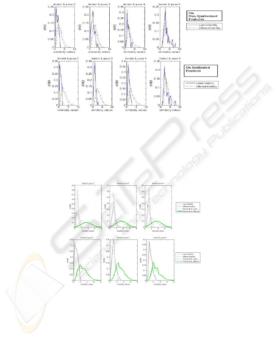
Fig. 4. x-axis denotes the similarity measure ‘γ’ and y-axis denotes the density approximation.

row depicts histograms for the same and different classes on non-synthesized features across

4 pose mismatches (see figure 1 for the approx. pose angles). 2

row depicts the kind of

separation and improvement we get by using feature synthesis.

As depicted in figure 5, the kernel density estimate is a better fit, this is because the

assumption of Gaussian distribution in such scenarios is generally not fulfilled.

Kernel density estimator, on the other hand, is known to approximate arbitrary

distributions [16].

Fig. 5. 1

row shows fitting a normal density, 2

row shows the kernel density fits on the

distribution of similarities obtained previously.

128128

3 Recognition Across Pose

Obtained likelihood estimates

pg p

(|S, )

γφ

and

pg p

(|D, )

γφ

, in the previous section,

can now be directly used to compute the posterior probability. For a probe image I

pose ‘

’, of unknown identity, we can now decide if it is coming from the same

subject as gallery I

, with each of the gallery image, by using this posterior as a

match score.

Employing these likelihoods, using Bayes rule, we write:

(12)

Since the pose

of the probe image is in general not known, we can marginalize

over it. In this case the conditional densities for similarity value

can be written as

(13)

(14)

Similar to the posterior defined in equation 12, we can compute the probability of

the unknown probe image coming from the same subject (given similarity

) as

(15)

If no other knowledge about the probe pose is given, one can assume the pose prior

) to be uniformly distributed. We, however, use the pose estimates for a given

probe face by our developed front-end pose estimation procedure [13]. Our pose

estimation system provides us with probability scores for each pose that can be used

directly as priors in equation 15. Due to a reasonably high accuracy of our pose

estimates, these probabilities can act as very strong priors and thus increase the

chances of a probe to be recognized correctly.

We compute this posterior for an unknown probe image with all of the

gallery

images and choose the identity of the gallery image with the highest score as

recognition result.

4 Recognition Results

As mentioned earlier, we use half of the subjects (34) in PIE database for training the

models described in the previous section, while images of remaining 34 subjects are

used for testing. As the gallery, the frontal images of all the 68 subjects are used. Note

that, since we do not assume any alignment between gallery and probe images,

therefore models are trained for the main 9 poses i.e. pose 1-9 in figure 1. While pose

10,11,12 and 13 corresponding to up/down tilt of the face are treated as the variations

due to misalignment for corresponding poses in the test set. All 13 poses for a subject

in the test set are therefore considered.

129129

Our results show that using our method one can achieve comparable results

without putting any hard constraints on alignment of facial parts. We, however,

include the Eigenface algorithm [11] for comparison, as it is the common benchmark

in facial image processing.

For our first experiment we assume the pose of the probe images to be un-known.

We therefore use equation 15 to compute the posterior probability that probe and

gallery images come from the same subject, where we use priors P(S)<<1 and

P(D)=1-P(S).

For an incoming probe image, we extract features as described in section 2.2. In

order to synthesize these features to frontal we need to know the probe pose, as we

have to use the corresponding pose transformation matrix B. Since we use a front-end

pose estimation step, as described in previous section that provides us with the

probabilities for different possible poses, we can directly use equation 13 and 14 by

transforming the extracted feature vector of given probe to frontal for all poses. As

these pose prior probabilities P(

) act as weights and since they are only high for the

nearest poses, therefore this does not affect the recognition performance much.

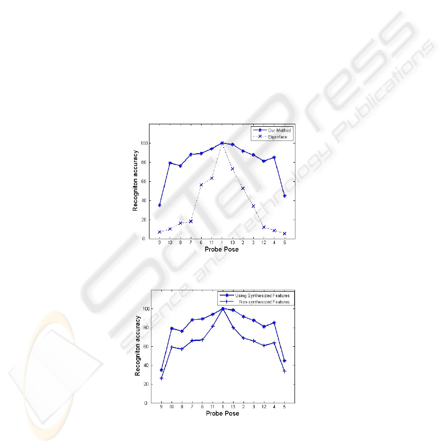
Figure 6 summarizes the recognition performance for each of the 13 poses for the

test set.

Fig. 6. Recognition results for our method and Eigenface for unknown probe pose, using

estimated pose probabilities (P(

)) as priors.

Fig. 7. comparison between recognition results of our method for with and without feature

synthesis.

130130

For the second experiment, we compare the performance with and without feature

synthesis. Figure 7 shows the performance gain achieved by using feature synthesis.

As much as 20 % of performance gain is observed for probe poses moving away from

frontal.

Note that when a probe is at frontal (pose 1), the scores are 100% since exactly the

same images are used in the gallery for frontal pose.

5 Discussion and Conclusions

Keeping in view the preceding discussion, we can now make some comments on the

performance of our method. Note in figure 6 and 7, as the probe pose moves away

from frontal, the scores deteriorate. The larger the width at which scores remain high,

the more pose invariant the algorithm is. The scores here are presented for the more

practical situation where the probe pose angles are not assumed known a priori. In

order to cope with that, we use marginalization over probe poses. However, since we

use feature synthesis, we need strong priors for the pose angles as opposed to using

uniformly distributed assumption i.e.

P( ) =

(for the 13 poses). As these priors act

as weights while computing the posterior in equation 15, using equal priors for every

pose results in degrading recognition performance. It is because an incoming probe

feature vector has to be transformed first to every pose using corresponding pose

transformation matrix. We have therefore used a front end pose estimation step,

which provides us with probabilities scores for each pose.

The clear advantage of using feature synthesis is shown by comparing recognition

performance with and without synthesis in figure 7. On concluding remarks, we have

presented a pose invariant face recognition method centered on modeling joint

appearance of gallery and probe images across pose in a Bayesian framework. We

have proposed novel extensions in this direction by introducing to use a more robust

feature description as opposed to pixel-based appearances. Using such features we

have proposed to synthesize the non-frontal views to frontal. The clear advantage of

this has been demonstrated experimentally. Furthermore using kernel density

estimate, instead of commonly used normal density assumption, is proposed to derive

the prior models. Our method does not require any strict alignment between gallery

and probe images and that makes it particularly attractive as compared to the existing

state of the art methods. Improved recognition across a wide range of pose has been

achieved using these extensions.

Although, we have presented results by using gallery as fixed at frontal pose, we

note that it is straight forward to use our method for any pose as gallery.

References

1. Beymer D.: Pose-invariant face recognition using real and virtual Views. M.I.T., A.I.

Technical Report No.1574, March 1996.

131131

2. Blanz V. and Vetter T.: Face recognition based on fitting a 3D morphable model. IEEE

Trans. PAMI, vol. 25, no. 9, 2003.

3. Brunelli R. and Poggio T.: Face recognition: Features versus templates. IEEE Trans.

PAMI, vol. 15, no. 10, pp. 1042–1052, 1993.

4. Gross R., Matthews I. and Baker S.: Appearance-based face recognition and light-fields.

IEEE Trans. PAMI, vol. 26, pp. 449–465, April 2004.

5. Kanade T. and Yamada A.: Multi-subregion based probabilistic approach towards pose-

invariant face recognition. in IEEE CIRA, vol. 2, pp. 954–959, 2003.

6. Kim T. and Kittler J.: Locally linear discriminant analysis for multimodally distributed

classes for face recognition with a single model image. IEEE Trans. PAMI, vol. 27, pp.

318–327, March 2005.

7. Lee H.S., Kim D.: Generating frontal view face image for pose invariant face recognition.

PR letters vol.27, No. 7, pp 747-754. 2006.

8. Lindeberg T.: Feature detection with automatic scale selection. Int. Journal of computer

vision, vol. 30 no. 2, pp 79-116, 1998.

9. Lowe D.: Distinctive image features from scale-invariant keypoints. Int. Journal of

computer vision, 2(60):91-110, 2004.

10. Martınez A. M.: Recognizing imprecisely localized, partially occluded, and expression

variant faces from a single sample per class. IEEE Trans. PAMI, vol. 24, no. 6, pp. 748–

763, 2002.

11. Moghaddam B. and Pentland A.: Probabilistic visual learning for object recognition. IEEE

Trans. PAMI, vol. 19, no. 7, pp. 696–710, 1997.

12. Mikolajczyk and Schmid C.: Performance evaluation of local descriptors. PAMI,27(10):31-

47, 2005.

13. Sarfraz M.S., Hellwich O.: Head pose estimation in face recognition across pose scenarios.

Int. conference on computer vision theory and applications VISAPP, 22-25 Jan, 2008.

14. Sarfraz M.S., Hellwich O.: Performance analysis of classifiers on face recognition", 5

IEEE AICS, pp. 255-264, 2006.

15. Sim T., Baker S., and Bsat S.: The CMU Pose, Illumination and Expression (PIE) database.

IEEE FG, pp. 46-51, 2002.

16. Silverman BW., Density estimation for statistics and data analysis. Chapman and Hall. 1992.

17. Vasilescu MA. O. and Terzopoulos D.: Multilinear analysis of image ensembles:

TensorFaces. ECCV, vol. 2350, pp. 447–460, 2002.

132132