
Shape Modeling for the Analysis of Heart Deformation
Patterns
Davide Moroni
1
, Sara Colantonio
1
, Ovidio Salvetti
1
and Mario Salvetti
2
1
Institute of Information Science and Technologies (ISTI)
Italian National Research Council (CNR), Pisa, Italy
2
Department of Mathematics, University of Pisa, Pisa, Italy
Abstract. In this paper, we present an approach to the description of time-varying
anatomical structures. The main goal is to compactly but faithfully describe the
whole heart cycle in such a way to allow for deformation pattern characterization
and assessment. Using such an encoding, a reference database can be built, thus
permitting similarity searches or data mining procedures.
1 Introduction
In the field of computer vision, analyzing the deformation pattern of non-rigid structures
may convey useful information in a variety of settings. For example satellite image
sequences display temporal evolution of complex structures like clouds and vortices,
whose analysis is essential for meteorological forecast [1]; reinforcement of speech
recognition by visual data may also be based on the analysis of lips deformation [2].
More interestingly for our purposes, in medicine, the detection and analysis of organ
deformations may shed new light in understanding their functional properties and may
convey non trivial support in diagnosis. Deformations inside the body may be inherent
to the nature of an organ (e.g. the lungs and the heart) or may be due to physiologi-
cal/pathological growth of tissues and structures. For example, it has been proven that
irregular growth of the hippocampus is strongly correlated to epilepsy; thus analysis
of hippocampus deformations through 3D models may be used as a clinical decision
support to avoid unnecessary brain surgery [3]. Again, in the field of neurology, simu-
lation of intracranial phenomena such as haemorrhages, neoplasm and hematoma may
be used to analyze the influences they have on neuro-functional structures in the brain
[4].
Imaging modalities provide an invaluable aid in analyzing such complex structures.
However image sequences contain a huge amount of high dimensional data (2 or 3 spa-
tial dimensions plus time) which cannot be fully exploited unless with the help of suit-
able tools for image processing, pattern recognition and image understanding. Actually,
in cardiac analysis, well-established imaging techniques (MRI, fastCT, PET, SPECT,
ultrasound, . . . ) allow to acquire video sequences of the heart, from which its dynami-
cal behavior can be inferred. However, in daily practice, sometimes, physicians extract
only the most salient frames from the video sequence (end diastole and systole) and
Moroni D., Colantonio S., Salvetti O. and Salvetti M. (2008).
Shape Modeling for the Analysis of Heart Deformation Patterns.
In Image Mining Theory and Applications, pages 37-50
DOI: 10.5220/0002341200370050
Copyright
c
SciTePress

perform direct comparison among images in the selected subset. Considering the full
video sequence, more precise and rich information about the state of the heart can be
actually discovered.
In this frame, cardiac modelling provides powerful methods for pattern analysis.
An abstract representation of the heart is built and can be instantiated to the particular
anatomy under examination, with the aim of extracting shape and functional param-
eters. In addition, cardiac modelling can enable sophisticated quantitative assessment
of heart pathologies, for which up-to-now only semi-quantitative evaluation is used in
clinical practice. For example, this is the case of ventricular dyssynchrony, a complex
phenomenon whose origins are to be tracked back to electrical conduction disturbances
that affect both regional and global function of the heart; dyssynchrony results into inco-
ordinate ventricular wall motion due to activation delay. Despite its relevance, the only
dyssynchrony marker that has received some consensus is an ECG-derived parameter,
which however is poorly correlated to the outcome of resynchronization therapy. It may
turn out that cardiac modelling may offer new insight into the problem of dyssynchrony
characterization, by conveying novel representation features and suitable tools for their
scientific visualization. Ultimately, dyssynchrony characterization may be translated
via the extracted features into a statistical pattern recognition problem, thus allowing
for new methods of quantification [5].
The main goal of cardiac modelling is to compactly but faithfully describe de-
formable structure in such a way to allow for deformation pattern characterization and
assessment. Such an encoding would be useful to build up a reference database for
similarity searches or data mining procedures.
Motivated by these problems and extending the works [6], [7] and [8], we first de-
fine in some generality, the concept of periodically deforming structures (see section
2 for a precise definition) and we start a methodological approach to their study. Be-
sides providing modules for structures reconstruction (Section 4) and characterization
(Section 5), that have their own importance in biomedical applications as automatic
tools to speed up diagnosis, the main idea is to define a reference dynamic model of
a structure class: this model can be understood as an encoding of morphological and
functional properties of a periodically deforming structure during its full deformation
cycle (Section 6). In particular, shape changes and evolution of local structure proper-
ties are depicted in a coincise form in the reference dynamic model, thus allowing for
deformation analysis and deformation pattern classification. The methodology is finally
applied to the analysis of heart left ventricle in magnetic resonance image sequences.
2 Periodically Deforming Structure
A structure O embedded in the background space Ω ⊂ R
d
(d = 2, 3) is a collection
O = {(V
α
, P
α
)}
α=1,2,...,k
where each V
α
is a smooth manifold (possibly with boundary) embedded in Ω and
P
α
: V
α
→ R
d(α)
is a smooth properties function assuming its values in a suitable
properties space.
The smoothness assumption is a quite common hypothesis in computational anatomy
3838

(see e.g. [9]) and it is satisfied in practice to a large extent; it implies for example
that differential geometric properties can be computed everywhere. We use, moreover,
collection of manifolds -instead of a single one- to be able to describe structure sub-
parts (possibly of different dimensionality) by attaching them specific salient attributes
via a dedicated properties function. For example, in heart left ventricle modeling, the
structure of interest is the myocardium, that can be modeled as a 3D manifold, whose
boundaries are two surfaces: the epicardium and the endocardium. It is convenient to
attach to the boundary surfaces a different (actually richer) set of attributes than those
used for internal points.
A deforming structure O = (O
t
)
t=0,1,...
is a temporal sequence of structures satis-
fying some smoothness constraints. Each O
t
= {(V
α
, P
α
)}
1≤α≤k
should be regarded
as the snapshot of the deforming structure at time t.
We require that each manifold V
α
t
appearing in the snapshot at time t can be smoothly
deformed into V
α
t+1
in the subsequent snapshot. Tears or crack of any structure subpart
are, therefore, ruled out; moreover, in such a way, we avoid dealing with changes in
topology, that would require to model shape transitions. Such a task would be essen-
tial for example in meteorological applications, but is far beyond our present scopes in
biomedical problems.
Finally, a periodically deforming structure is a deforming structure for which there
exists an integer T such that ∀t : O
t
= O
t+T
. In other words, the deforming structure
depicts a periodic motion; thus, a periodically deforming structure is characterized by a
finite list of snapshots (O
0
, O
1
, . . . , O
T −1
), which will be referred to as its deformation
cycle.
We make a final assumption about the data available to describe a periodically de-
forming structure. It is assumed that a sufficiently rich set of synchronous signals and
images, possibly from different modalities, has been acquired so as to represent faith-
fully a physical body or phenomenon of interest. In particular, the data set should in-
clude at least one 2D/3D image sequence (S
t
)
0≤t≤T −1
, from which morphology and
regional properties of the structure can be inferred.
3 Outline of the Methodology
With the previous assumptions, a reference dynamic model of a structure of interest is
constructed by coding the dynamics of the structure in a concise representation of its
shape and functional properties.
The approach consists in three modules, each one performing specific tasks. Essentially,
the first two modules are dedicated to extract a suitable periodically deforming structure
from image data. Then the periodically deforming structure is analyzed and used to
construct the reference dynamic model. A more precise outline of the modules used to
obtain the aforementioned model is as follows:
Structure Reconstruction. For each phase t, the collection of manifolds {V
α
t
} is iden-
tified and reconstructed in 2D/3D space by applying neural algorithms to the image
sequence (S
t
)
1≤t≤T
;
Structure Characterization. Morphological features and dynamic descriptors are ex-
tracted and coded in a property function P
α
t
that for each point x of the manifold
3939

V
α
t
returns the property vector (P
α
1
(x), . . . , P
α
m
(x)), where each P
α
i
represents
one of the selected features;
Deformation Pattern Assessment. Suitable and significant shape descriptors are ex-
tracted and spatial distribution of the property functions are evaluated in order to
obtain a description of the structure dynamics.
In the following sections, these steps are described in more details.
4 Structure Reconstruction
We address the problem of deformable structure reconstruction with a two-stage method,
which, firstly, automatically localize the deformable structure and then extracts its finer
details, looking for precise contours of the whole structure and of its subparts. To each
image S
t
, the following two-stage procedure is applied:
1. Structure automatic localization: a cluster analysis, based on the fuzzy c-means
algorithm, is applied to identify and label homogeneous regions in each image.
Through a region tracking procedure, the behavior of these regions is analyzed
over an entire cycle, in order to extract a rough approximation O
0
= {O
0
t
}
0≤t≤T −1
of the deformable structure O.
2. Segmentation refinement: O
0
is used to compute the approximate orientation of the
real structure O, which, in turn, is used to extract three-dimensional features pro-
cessed by a dedicated ANN, in order to complete the segmentation, by identifying
accurate contours of O.
4.1 Automatic Localization of Deformable Structures
We assume that shape descriptors of the deformable structure tracked on time exhibit a
periodical behavior, with main frequency concentrated in the motion frequency. Further
we assume that the subparts of the deformable structures appear as homogeneous re-
gions at some scale. However the latter assumption is dictated by our implementations
and can be substituted without altering the spirit of this contribution.
Clustering. Homogeneous image regions are first labeled using an unsupervised clus-
tering method, based on the fuzzy c-means algorithm (FCM) [10]. This algorithm groups
a set of data in a predefined number of regions so as to iteratively minimize a crite-
rion function, namely the sum-of-squared-distance from region centroids, weighted by
a cluster membership function. A membership grade p ∈ [0, 1] is associated to each
element of the data set, describing its probability to be in a particular cluster.
The FCM algorithm is applied to each image S
t
to produce a number of clusters:
for any voxel x, a features vector (I
0
(x), I
1
(x), I
2
(x), . . . , I
r
(x)) is computed so that
I
0
(x) = S
t
(x), and for d = 1, . . . , r, we set I
d
(x) = G
d
∗S
t
(x), where G
d
is a Gaussian
kernel with standard deviation σ ∝ d.
This, in turn, induces a partition of the image domain into a set P
t
= {R
1
t
, R
2
t
, . . .}
of disjoint connected regions, where the upper indices 1, 2, . . . are region labels. In the
following, ρ
t
will denote the generic region in P
t
.
4040

Region Tracking. Once eliminated regions of negligible volume (island removal), an
intra-cycle tracking procedure is performed. A simple centroid-based tracking algo-
rithm associates, to any region ρ
t
∈ P
t
in the phase t, its correspondent region T (ρ
t
) ∈
P
t+1
in the subsequent phase t + 1. The procedure can be iterated, thus producing a
region sequence
ρ
t
= T
0
(ρ
t
) → T
1
(ρ
t
) → T
2
(ρ
t
) → . . .
which may be thought as the evolution of the starting region ρ
t
in the different phases.
Considering t = 0 as reference phase, for each ρ
t
∈ P
t
the regions appearing in its
evolution are collected in a list Ev(ρ
0
) = (T
t
(ρ
t
))
0≤t≤T −1
.
Features Extraction. For any region ρ
0
∈ P
0
, the behavior in time of a shape de-
scriptor G (such as elementary geometric properties: volume, inertia moments etc. )
can be estimated by evaluating G for every element in the list Ev(ρ
0
), thus obtain-
ing a vector f
G
(ρ
0
) = (G.T
t
(ρ
0
))
0≤t≤T −1
. We then switch to the frequency domain
to detect the oscillatory behavior of f
G
(ρ
0
). Actually, the first harmonic coefficient
ν
G
(ρ
0
) in the power spectrum density is selected as a salient feature. Indeed, for fixed
regions the variations in G during time are essentially due to noise; instead for re-
gions in periodic motion the spectrum power is concentrated in the motion frequency.
Finally, for a predetermined list {G, H, . . .} of shape descriptors, a features vector
I(ρ
0
) = (µ
G
(ρ
0
), ν
G
(ρ
0
), µ
H
(ρ
0
), ν
H
(ρ
0
), . . .) is associated to each ρ
0
∈ P
0
.
Region Classification. Let O
0
t
denote the region corresponding to the deformable struc-
ture O at the phase t. At first, the reference phase is considered and O
0
0
is searched
among regions ρ
0
∈ P
0
, taking into account their features vectors I(ρ
0
). More pre-
cisely, a set of learning examples is used to introduce a Mahalanobis distance in the
feature space. Let I
1
, I
2
, . . . I
s
be a set of observed feature vectors relative to a training
set of regions O
0
with mean m and covariance matrix Σ. The associated Mahalanobis
distance, defined by
D(I) =
(I − m)
t
Σ
−1
(I − m)
1/2
,
measures the dissimilarity of a feature vector w.r.t. to the expected region feature vector.
Thus, for any new case, O
0
0
is selected among candidate regions ρ
0
∈ P
0
according to
the criterion:
O
0
0
= arg min
ρ
0
∈P
0
D(I(ρ
0
))
In subsequent phases, the region O
0
t
is singled out by means of the tracking algorithm,
namely O
0
t
is defined as T
t
(O
0
0
).
4.2 Segmentation Refinement
The localization of the deformable structure in the previous section supplies as a byprod-
uct a rough approximation of its boundary surface, which may suffer from poor inten-
sity contrast or the presence of spurious structures. The aim of this stage is to refine the
segmentation found in the previous section and to identify as well the contours of the
4141

structure subparts.
The set up is as follows. Let Ω ⊂ R
3
be the image domain of the image S
t
. First we de-
fine a features function F : Ω → R
s
, that assigns to each point x ∈ Ω a vector F(x)
of local features extracted from the image data S
t
. Then we use an approach based
on Multi-Level Artificial neural networks (MANN) to find functions Φ
α
: R
s
→ R
(α = 1, 2, . . . , k) s.t. the level sets:
V
α
= {x ∈ Ω| Φ
α
(F(x)) = 0} α = 1, 2, . . . k (1)
correspond to the surface V
α
respectively.
The functions Φ
α
are learned using a training set of segmented images and they can be
used subsequently to segment new instances.
Features Extraction Given an image S
t
: Ω → R, a features function F : Ω → R
s
may be constructed. Since the neural network will eventually use this function for the
identification of image edges, it is clear that the function F should include edge indica-
tor clues.
The involved features can be divided into two classes. First, low-level features are con-
sidered: they are context-independent and do not require any knowledge and/or pre-
processing. Some examples are voxel position, gray level value, gradients and other
differentials, texture, and so forth. Middle-level features are also selected, since voxel
classification can benefit from more accurate clues, specific of the problem at hand. In
particular, the knowledge of the deformable structure orientation, obtained as a byprod-
uct in the localization procedure, can be used to individuate an Intrinsic Reference Sys-
tem (IRS) suitable to describe the structure shape. If, in addition, a priori information
about the structure shape is available, a reliable clue for detecting edges in the images is
given by the gradient along the normal direction to the expected edge orientation. More-
over, a multiscale approach is adopted: the features are computed on blurred images,
supplying information about the behavior of the voxel neighborhood, which results in a
more robust classification.
MANN-based Voxel Classification The set of selected features are processed to ac-
complish the voxel classification by means of a Multilevel Artificial Neural Network
(MANN), which assures several computational advantages [11]. For each voxel x, its
computed features vector F(x) is divided into vectors F
i
(x), each one containing fea-
tures of the same typology and/or correlated. Then each F
i
(x) is processed by a ded-
icated classifier based on an unsupervised Self Organizing Maps (SOM) architecture.
The set of parallel SOM modules constitutes the first level of the MANN which aims
at clustering each portion of the feature vector into crisp classes, thus reducing the
computational complexity. Cluster indexes, in turn, are the input of the final decisional
level, operated by a single EBP network. The output of this last module consists in
the vector (Φ
α
(F(x)))
1≤α≤k
describing voxel membership to the various surfaces V
α
(1 ≤ α ≤ k) according to Equation 1.
The SOM modules are trained according to the Kohonen algorithm [12]. For the
EBP module, a set of 3D images should be pre-classified by an expert observer and
used for supervised training, performed according to the Resilient Back-Propagation
algorithm [13].
4242

5 Structure Characterization
The reconstructed structure is further characterized by assigning a significant proper-
ties function P
α
t
: V
α
t
→ R
d(α)
to each manifold V
α
t
. Three types of properties are
considered:
– intensity based properties;
– local shape descriptors;
– local dynamic behavior descriptors.
Examples of properties of the first type are gray level value, gradients, textures and the
like. They are extracted form the image sequence S
t
–the one which leads us to structure
reconstruction. If data collected from other imaging modalities are available, after per-
forming registration, we can fuse this information to further annotate the structure (for
example, in the case of the heart, information regarding perfusion and metabolism, ob-
tained e.g. by means of PET imaging, can be referred to the reconstructed myocardium).
Geometric based properties, belonging to the second type, are extracted directly from
the collection of manifolds {V
α
t
}, and are essential to describe locally the shape of the
structure. Again, we may distinguish between context independent features (automat-
ically computable for every manifold of a given dimensionality, such as Gaussian and
mean curvature for surfaces) and problem-specific properties.
Finally, the local dynamic behavior may be described by properties borrowed from
continuous mechanics (such as velocity field and strain tensor); they, however, require,
at least, local motion estimation, that we haven’t pursued yet.
6 Deformation Pattern Assessment
The aim of this section is to provide methods for the representation of a deformable
structure which are suitable for similarity searches and data mining procedures. The
main idea is to combine the well established feature vector paradigm for 3D objects
(see e.g. [14] for a recent survey) with a modal analysis, able to cope with periodically
deforming structures.
Indeed, although the periodically deforming structure obtained in the previous steps
can be used in principle to assess the dynamic behavior of the structure and identify its
deformation pattern, the voxelwise characterization of the reconstructed structures is not
suited for similarity searches. The reason is twofold. First, the given description of the
whole structures (collection of manifolds described by functions) has a dimensionality
far too high to make the problem computationally feasible. Even worse, the voxelwise
characterization does not permit, at least in a straightforward manner, the comparison
of anotomical structures belonging to different patients or relative to different phases in
the cycle.
We addressed this issue using a deformable model (given for example by mass-spring
models as presented in [4] ) and normalizing every instance of anatomical structure
to that model: in this way anatomical structures (belonging to the same family) are
uniformly described and can be then compared according to the feature paradigm.
4343

To recap, we should look for a new set of ‘more intrinsic’ features F
t
that should be
enough simple and, at the same time, capturing essential information about the struc-
tures.
To obtain these new kind of features, global information about the structures can be ex-
tracted from the properties function, without introducing any problem-specific model.
For example, one may consider the property spectrum, that is, by definition, the prob-
ability density functions (PDF) of a given component of the property function P
α
t
(·).
This function captures how the property is globally distributed; thus, comparison of dif-
ferent property spectra is directly feasible; to reduce dimensionality, moreover, it could
be effective to compute the momenta of the PDF (mean, variance,. . . ).
However, properties spectrum does not convey any information at all about regional
distribution of the property. In clinical applications, this is a drawback which cannot
be ignored: actually a small highly abnormal region may not affect appreciably the
property spectrum, but its clinical relevance is, usually, not negligible. Hence, spatial
distribution of properties has to be analyzed. One approach would be to estimate mul-
tidimensional property spectrum [15]. In this way, we may implicitly encode spatial
relationship between different kind of features. For example, considering the cords go-
ing from the center of mass of a structure to its boundary, we may use the cord length
and orientation as a property function defined on the structure boundary. Then, the as-
sociated multidimensional PDF implicitly codifies the elongation axis of the structure.
A major issue in dealing with such sort of multidimensional shape distributions is the
accurate estimation of the PDF. Some methods, based on the fast Gauss transform, have
been reported [16]. Although, this approach may be conceivable for general-purpose
3D structure indexing and retrieval, it has low relevance in medical applications, for
the too implicit encoding and the scarce characterization capabilities of local abnormal
regions. In the same vein, approaches which do not need a refined model of the struc-
ture (e.g., Gaussian image, spherical harmonics, Gabor spherical wavelets and other
general purposes shape descriptors used for content-based image retrieval) may be suit-
able. However, in general one should define a model of the structures (whose primitives
-elementary bricks- are regions, patches or landmarks) and then propagate it to the set
of instances to be analyzed by using matching techniques. It is then possible to consider
the average of a property on regions or patches (or its the value in a landmark) as a good
feature, since comparisons between averages on homologous regions can be performed
straightforwardly.
Following this recipe, a vector of features F
t
with the desired properties is obtained
for each phase of the cycle. The deforming structure is then described by the dynamics
of the temporal sequence of feature vectors obtained at different phases of the deforma-
tion cycle.
A further fruitful feature transformation may be performed exploiting our assump-
tions on deformable structures. Indeed, the smoothness of deformations implies that a
structure has mainly low frequency excited deformation modes. We extend this slightly
assuming that this holds true also for the features lists (F
t
)
1≤t≤T
. We assume that the
fundamental frequency of the motion is also the main component of each feature tracked
on time. With these assumptions, an obvious choice is given by the Fourier transform,
followed by a low pass filter, which supplies a new features vector Θ.
4444
frame 0 frame 1 frame 2 frame 3 frame 4
frame 5 frame 6 frame 7 frame 8 frame 9
frame 10 frame 11 frame 12 frame 13 frame 14
frame 15 frame 16 frame 17 frame 18 frame 19
frame 20 frame 21 frame 22 frame 23 frame 24
frame 25 frame 26 frame 27 frame 28 frame 29
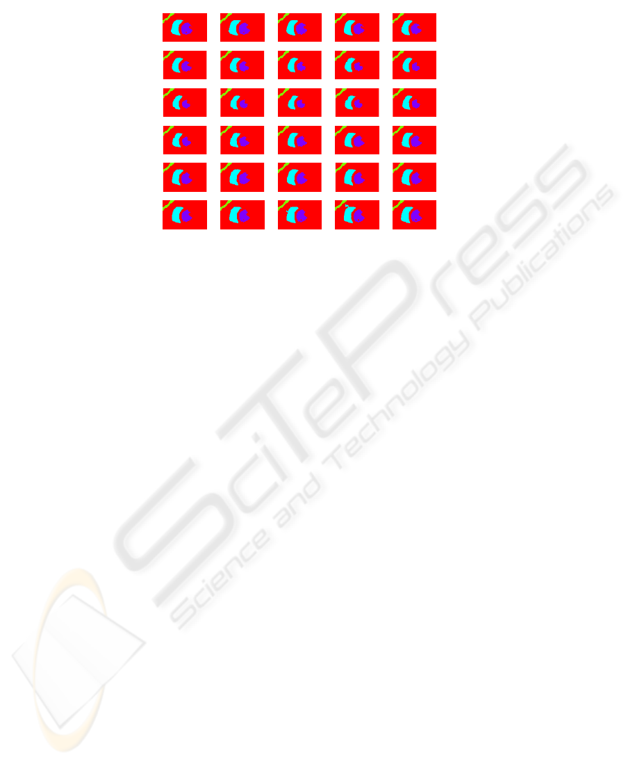
Fig. 1. Visualization of the results of clusterization and tracking algorithm (slice number 5).
The evaluation of the above mentioned parameters F
t
, at each phase t, implicitly
codifies information regarding structure dynamics.
7 Case Study: Heart Left Ventricle Analysis
An elective case study for the presented methodology is the analysis of Left Ventricle
(LV) that, pumping oxygenated blood around the body, is the part of the heart for which
contraction abnormalities are more clinically significant.
The LV structure is modeled as a 3D manifold (the myocardium) with boundary.
The boundary has two connected components which are the surfaces corresponding to
epicardium and endocardium.
We describe henceforth how the steps of the methodology are applied. First, the de-
formable structure is extracted from the available data, consisting in a sequence of short
axis gradient echo MR images, acquired with the FIESTA, GENESIS SIGNA MRI de-
vice (GE medical system), 1.5 Tesla, TR = 4.9 ms, TE = 2.1 ms, flip angle 45
◦
and
resolution (1.48 × 1.48 × 8) mm. Sets of T = 30 3D images, consisting of k = 11 2D
slices, were acquired at the rate of 30 ms for cardiac cycles [diastole-systole-diastole].
Various clinical cases were considered, for a total of 360 images, corresponding to 12
cardiac cycles. First, FCM was applied separately to each image to produce two clus-
ters using 2 as fuzziness parameter; we considered as a feature vector (I
0
, I
1
, . . . , I
r
)
where I
d
= G
d
∗S
t
and G
d
is a gaussian kernel of standard deviation d times the inslice
resolution.
Experimental testing showed that setting r = 2 is sufficient to get a good partition of
the image domain. The result of the tracking procedure on a middle slice is shown in
Figure 1.
The convex-hull volume and the inertia moments were considered as geometric
properties. The use of convex volume (instead of the simpler volume) reduces the effect
4545
of papillary muscles that sometimes move towards the boundary of the region corre-
sponding to the LV. Processing was performed only on middle slices, thus eliminating
the apical cap and the basal segments of the LV. Analysis of various clinical cases has
been used to introduce the Mahalanobis distance D; for simplicity, the covariance ma-
trix Σ has been assumed to be diagonal.
The previously found region corresponds roughly to the LV cavity (LVC) and may
be used to introduce an IRS. Since LV is essentially bullet shaped, a hybrid spher-
ical/cylindrical reference system is suitable to characterize its geometry and extract
salient edge information. To describe more in detail the IRS, suppose, without loss of
generality, that the z-axis of Ω ⊂ R
3
coincides with the long axis of the LV com-
puted in the previous section and that it is oriented from the apex to the base of the
LV. A point O = (0, 0, z
0
) on the long axis is selected as the switching point between
cylindrical and spherical coordinates. Cylindrical coordinates (r, θ, h) are assigned to
points x = (x, y, z) ∈ R
3
satisfying z − z
0
≥ 0, whereas spherical coordinates
(r, θ, φ) are given to points satisfying z − z
0
≤ 0. Notice that the unit vector field
ˆr(x) =
∂
∂r
x/||
∂
∂r
x|| (pointing in direction of increasing radial coordinate r) is almost
orthogonal to cardiac surfaces and, therefore, the derivative
∂S
t
∂r
along the radial direc-
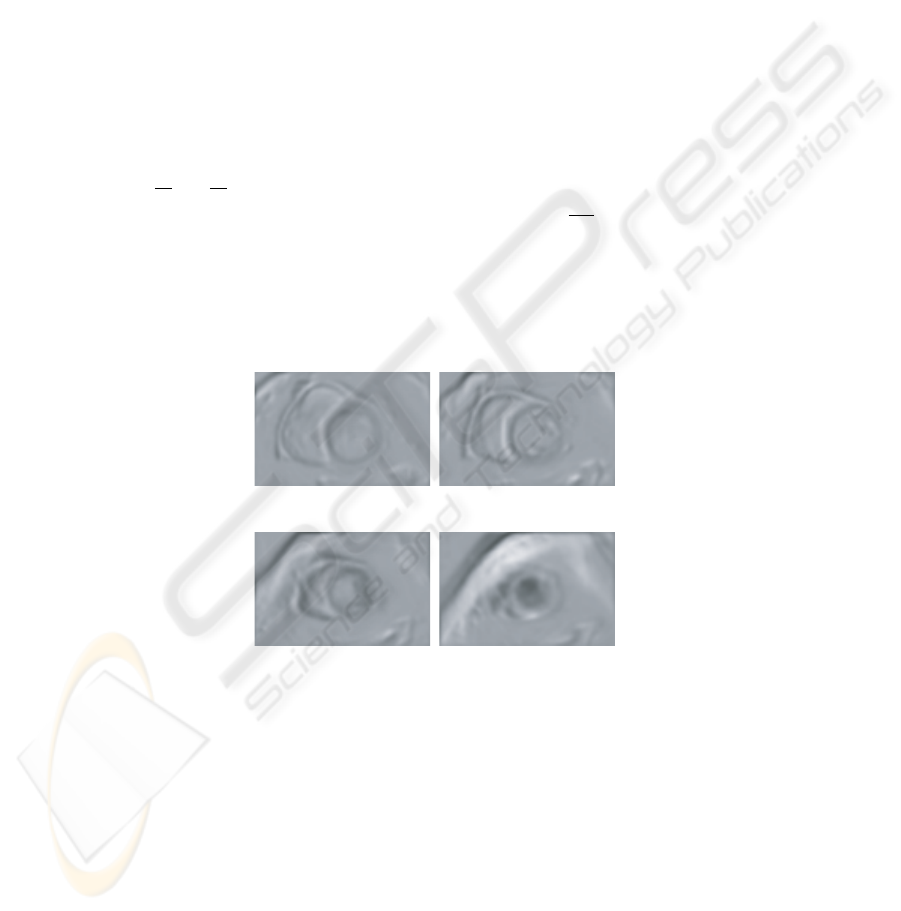
tion may be used as a clue for edge detection. Indeed for a point on a cardiac surface, the
modulus of radial derivative is likely to be a high fraction of total gradient magnitude
(see Figure 2). Moreover the degree of freedom in the choice of the switching point O
may be used to tune the IRS to the peculiar cardiac geometry under exam.
(a) Slice 3 (b) Slice 5
(c) Slice 7 (d) Slice 9
Fig. 2. Example of computed features: radial derivative.
The hybrid reference system is used to associate to each point x = (x, y, z) ∈ Ω, a
vector consisting of the following features extracted from the data :
– Position. The position of a point x w.r.t. the IRS is expressed as a quadruple
(r, θ, φ, h). If z − z
0
≤ 0 the entries r, θ, φ represent its spherical coordinates,
whereas h is set to 0. Similarly, for z − z
0
≥ 0, the entries r, θ, h represent its
4646

cylindrical coordinates whereas φ is set to π/2. Notice that with this choice both
definitions agree for points in the plane z = z
0
.
– Intensity. The intensity value S
t
(x) as well as its smoothed analogues G
d
∗S
t
(x).
– Gradient norm. Gradient norm||∇(G
d
∗S
t
(x))(x)|| of the smoothed imagesG
d
∗S
t
.
– Radial derivative. The radial derivative of the smoothed images
∂G
d
∗S
t
(x)
∂r
(x) =
∇(G
d
∗S
t
(x)) · ˆr.
Using the 2-level ANN, voxels are classified on the basis of their features vector as be-
longing or not to epi- and endocardial surfaces. More in detail, the set of extracted fea-
tures is divided into two vectors F
1
, F
2
containing respectively 1) position and intensity
and 2) position, gradient norm and radial derivative. The position w.r.t. IRS is replicated
in both vectors because it reveals salient for clustering both features subsets. Then, the
first level of the MANN consists of two SOM modules, which have been defined as 2D
lattice of neurons and dimensioned experimentally, controlling the asymptotic behav-
ior of the number of excited neurons versus the non-excited ones, when increasing the
number of total neurons [17].
A 8 × 8 lattice SOM was then trained for clustering the features vector F
1
, while
F
2
was processed by a 10 × 10 lattice SOM.
A single EBP module has been trained to combine the results of the first level and
supply the final response of the MANN. The output layer of this final module consists
in two nodes, which are used separately for reconstructing the epicardium and the endo-
cardium. Since each cardiac surface divides the space into two connected regions (one
of which is bounded), each output node can be trained using the signed distance func-
tion with respect to the relative cardiac surface. In this way, points inside the surface are
given negative values, whereas positive values are given to points in the outside. Hence-
forth the surface of interest correspond to the zero-level set of the output function.
Different architectures have been tested, finding the best performance for a network
with only one hidden layer of 15 units. A manual segmentation was performed with ex-
pert assistance on the available data. A set of 240 images was used for network training,
while the remaining ones were used for network performance test.
The voxel classification, supplied by the MANN, may be directly used for visual-
ization purposes by using an isosurface extraction method, as shown in Figure 3. Figure
4 shows the intersection of the two cardiac surfaces with a slice plane.
Characterization of the reconstructed structure is obtained annotating every voxel
with intensity, Gaussian and mean curvature, wall thickness and IRS properties. In par-
ticular, Gaussian and mean curvature have been included as shape descriptors whereas
wall thickness, which is a classical cardiac parameter, is one example of problem-
specific property: it is defined as the thickness of the myocardium along a coordinate
ray and it is expected to increase during contraction, since myocardium, being almost
water, is, with good approximation, incompressible (see Figure 5).
This characterization is translated into a more amenable form by computing proper-
ties spectrum and regional features. In computing spectrum, coordinates w.r.t. IRS have
been disregarded, with the exception of radial coordinate; intensity has also been ex-
cluded. For any property only mean and variance have been considered. For computing
regional features, so far, we used a popular model of the LV (see [18] for a review of
3D-cardiac modelling). In 2D, as shown in Figure 6, it is defined by the intersections of
4747
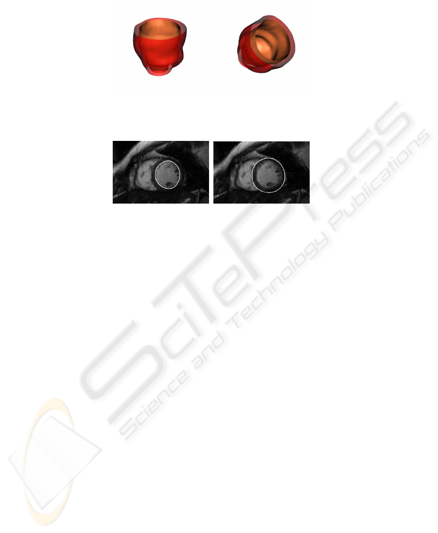
Fig. 3. Different views of the rendered left ventricle at end diastole. The surfaces are obtained
applying marching cubes on the two output functions of the network. To eliminate satellites, a
standard island removing procedure is applied.
(a) Endocardium (b) Epicardium
Fig. 4. Intersection of cardiac surfaces with a slice plane.
cardiac surfaces with a pencil of equally spaced rays.
The 3D version is obtained by stacking the 2D construction along the axis of the LV.
Only 7 middle slices have been considered, giving a total of 168 model points.
The final feature vector Θ is obtained taking the first two harmonics of the Fourier
transform of the time-sequence (F
t
)
0≤t≤T −1
. Since 5 real parameters are required to
describe a signal up to second harmonic, the compression ratio is 6 : 1.
8 Conclusions and Further Work
In this paper, we have defined a reference dynamic model, encoding morphological
and functional properties of a structures class, capable to analyze different scenarios in
heart left ventricle analysis. In particular, a framework for the shape characterization
and deformation analysis has been introduced for the study of periodically deforming
structures.
This framework consists of several modules performing a) structure reconstruction,
b) structure characterization, c) pattern deformation assessment. Solutions to specific
tasks proposed in each module are, to a large extent, independent and may be combined
with other methods, thus broadening the potential application field of the framework. In
particular, an approach based on multi-level artificial neural networks has been selected
as a general purposes strategy for structure reconstruction, motivated by the promising
results presented in [11]. A quantitative evaluation of segmentation performance, based
on comparison between images automatically segmented and images annotated by a
committee of expert observers, however, is still in progress.
4848
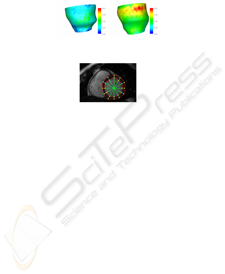
Fig. 5. Wall thickness at end diastole and systole, shown as an attribute of epicardial surface. Es-
timation is performed according to the centerline method and values are expressed in millimeters.
Fig. 6. The pencil of equally spaced rays used to computed local features.
The elective case studies are represented by the analysis of heart deformable anatom-
ical structures. Actually, for demonstrating the effectiveness of the proposed framework,
we have shown the preliminary results in the study of the heart left ventricle dynamics.
The next step will be to employ the obtained results for building up a reference database
for similarity searches or data mining procedures.
Acknowledgements
This work was partially supported by European Project Network of Excellence MUS-
CLE - FP6-507752 (Multimedia Understanding through Semantics, Computation and
Learning) and by European Project HEARTFAID “A knowledge based platform of ser-
vices for supporting medical-clinical management of the heart failure within the elderly
population”(IST-2005-027107).
References
1. Papin, C., Bouthemy, P., M
`
emin, E., Rochard, G.: Tracking and characterization of highly
deformable cloud structures. In: Computer Vision - ECCV 2000. Volume 1843 of LNCS.,
Springer Verlag (2000) 428–442
2. Bregler, C., Konig, Y.: “Eigenlip” for robust speech recognition. In: Acoustics, Speech, and
Signal Processing ICASSP-94. Volume II. (1994) 669–672
3. Keim, D.: Efficient geometry-based silmilarity search of 3D spacial databases. In: Proceed-
ings of the 1999 ACM SIGMOID, New York, ACM Press (1999) 419–430
4. Di Bona, S., Lutzemberger, L., Salvetti, O.: A simulation model for analyzing brain struc-
tures deformations. Physics in Medicine and Biology 48 (2003) 4001–4022
4949

5. Boyer, K.L., Gotardo, P.F.U., Saltz, J.H., Raman, S.V.: On the detection of intra-ventricular
dyssynchrony in the left ventricle from routine cardiac mri. In: ISBI. (2006) 169–172
6. Colantonio, S., Moroni, D., Salvetti, O.: Shape comparison and deformation analysis in
biomedical applications. In: Eurographics Italian Chapter Conference. (2006) 37–43
7. Moroni, D., Perner, P., Salvetti, O.: A general approach to shape characterization for biomed-
ical problems. In Perner, P., ed.: Industrial Conference on Data Mining ICDM - Workshop
on Mass-Data Analysis of Images and Signals. IBAI CD-Report, Leipzig (2006) 56–65
8. Moroni, D., Colantonio, S., Salvetti, M., Salvetti, O.: Deformable structures localization and
reconstruction in 3D images. In Ranchordas, A., Araujo, H., Vitria, J., eds.: 2nd International
Conference on Computer Vision Theory and Applications. INSTICC, Barcelona (2007) 215–
222
9. Grenander, U., Miller, M.I.: Computational anatomy: an emerging discipline. Q. Appl. Math.
LVI (1998) 617–694
10. Bezdek, L.: Pattern Recognition with Fuzzy Objective Function Algorithm. Plenum Press,
New York (1981)
11. Di Bona, S., Niemann, H., Pieri, G., Salvetti, O.: Brain volumes characterisation using
hierarchical neural networks. Artificial Intelligence in Medicine 28 (2003) 307–322
12. Kohonen, T.: Self-Organizing Maps. 2nd edn. Volume 30 of Springer Series in Information
Sciences. (1997)
13. Riedmiller, M., Braun, H.: A direct adaptive method for faster backpropagation learning: The
RPROP algorithm. In: Proc. of the IEEE Intl. Conf. on Neural Networks, San Francisco, CA
(1993) 586–591
14. Bustos, B., Keim, D.A., Saupe, D., Schreck, T., Vranic, D.V.: Feature-based similarity search
in 3d object databases. ACM Comput. Surv. 37 (2005) 345–387
15. Akg
¨
ul, C.B., Sankur, B., Schmitt, F., Yemez, Y.: Multivariate density-based 3d shape de-
scriptors. In: Shape Modeling International. (2007) 3–12
16. Akg
¨
ul, C.B., Sankur, B., Yemez, Y., Schmitt, F.: Improving efficiency of density-based shape
descriptors for 3d object retrieval. In: MIRAGE. (2007) 330–340
17. Di Bono, M., Pieri, G., Salvetti, O.: A tool for system monitoring based on artificial neural
networks. WSEAS Transactions on Systems 3 (2004) 746–751
18. Frangi, A.F., Niessen, W.J., Viergever, M.A.: Three-dimensional modeling for functional
analysis of cardiac images: A review. IEEE Trans. Med. Imaging 20 (2001) 2–5
5050
