
Mutual Calibration of a Camera and a Laser
Rangefinder
Vincenzo Caglioti, Alessandro Giusti and Davide Migliore
Politecnico di Milano, Dipartimento di Elettronica e Informazione, Italy
Abstract. We present a novel geometrical method for mutually calibrating a
camera and a laser rangefinder by exploiting the image of the laser dot in relation
to the rangefinder reading.
Our method simultaneously estimates all intrinsic parameters of a pinhole natural
camera, its position and orientation w.r.t. the rangefinder axis, and four parame-
ters of a very generic rangefinder model with one rotational degree of freedom.
The calibration technique uses data from at least 5 different rangefinder rota-
tions: for each rotation, at least 3 different observations of the laser dot and the
respective rangefinder reading are needed. Data collection is simply performed
by generically moving the rangefinder-camera system, and does not require any
calibration target, nor any knowledge of environment or motion.
We investigate the theoretical limits of the technique as well as its practical ap-
plication; we also show extensions to using more data than strictly necessary or
exploit a priori knowledge of some parameters.
1 Introduction
We consider a rangefinder-camera system and a solidal frame of reference F ; the range-
finder itself can rotate around a generic axis solidal to F . After the mutual calibration
is completed, we can:
– recover the viewing ray (in the reference frame F ) associated to any image point
(camera calibration);
– recover the measuring ray (in the reference frame F ) associated to any rangefinder
angle, and a point on this ray which returns a zero reading (rangefinder calibration).
Mutual rangefinder-camera calibration is needed for relating rangefinder readings to
the respective image points; this is a prerequisite for correlating rangefinder and image
data, which is useful for many practical tasks such as obstacle detection and characteri-
zation, 3D shape and texture reconstruction, robot self-localization, odometry and map-
ping. Our proposed solution does not require any specific calibration object, and can be
performed automatically by just sampling rangefinder readings and camera images dur-
ing generic relative motion of the rangefinder-camera system or the surrounding scene:
the only requirement is that you get at least three different range readings for each of
five different rangefinder angles.
Caglioti V., Giusti A. and Migliore D. (2008).
Mutual Calibration of a Camera and a Laser Rangefinder.
In VISAPP-Robotic Perception, pages 33-42
DOI: 10.5220/0002341700330042
Copyright
c
SciTePress

The problem is hard since it is characterized by many variables and degrees of free-
dom, related to the camera characteristics, camera position, and rangefinder construc-
tion. In its most general form, the problem assumes almost no knowledge on the system
characteristics and environment parameters; on the other hand, each of our observations
is very basic and it only consists in a point on the image and the related rangefinder
reading. When compared to the problem of calibrating a camera alone without any
prior knowledge of the environment (autocalibration), our technique is surprising for its
simplicity, expecially if accounting for the additional degrees of freedom which char-
acterize this scenario. This is intuitively explained by considering that our technique
exploits some properties of the rangefinder function (such as the linearity of the mea-
suring ray): therefore, while being calibrated, it also provides constraints for camera
calibration, and vice-versa. An intersting related work from this point of view is [8],
which calibrates a camera using a laser pointer as a calibration device.
Our work heavily relies on known techiques in projective geometry [5]. In particu-
lar, our camera calibration technique is related to the method introduced by Colombo
et al. in [2], which calibrates a camera using coaxial circles; other interesting alge-
braical properties of coplanar circles for camera calibration and 3D structure extraction
are presented in [4, 6]. The problem of simultaneously calibrating a camera and a laser
rangefinder has been recently challanged with several approaches: in [9], a checker-
board calibration pattern is used, and its images and distance profiles are related in
order to find the camera position and orientation w.r.t. the rangefinder; in [1] a special
3D calibration object allows to automatically calibrate a laser rangefinder. Our tech-
nique is different in that it does not use any explicit calibration target, but exploits the
visible image of the laser dot; a similar approach is found in [7], where some alge-
braic constraints on the camera-rangefinder calibration due to the laser dot visibility are
derived.
In Section 2 we formally define the problem and its parameters and variables. Sec-
tion 3 presents our technique, and sketches the extension to 2-DOF rangefinders. Sec-
tion 4 discusses the results, and proposes variations for calibrating only a subset of the
parameters, and using more data than strictly needed.
2 Definitions, Model and Data
2.1 System Model
We consider a camera-rangefinder system; the rangefinder has 1 rotational DOF around
a generic axis; the rangefinder rotation angle φ is not calibrated – i.e., the actual angle
is not necessarily known, but repeatable.
We define a reference frame F as follows:
– F
z
coincides with the rangefinder rotation axis;
– F
x
is parallel to the projection on the xy plane of the rangefinder ray when φ = 0;
– the origin is placed at the nearest point on the rotation axis to any telemeter ray.
3434
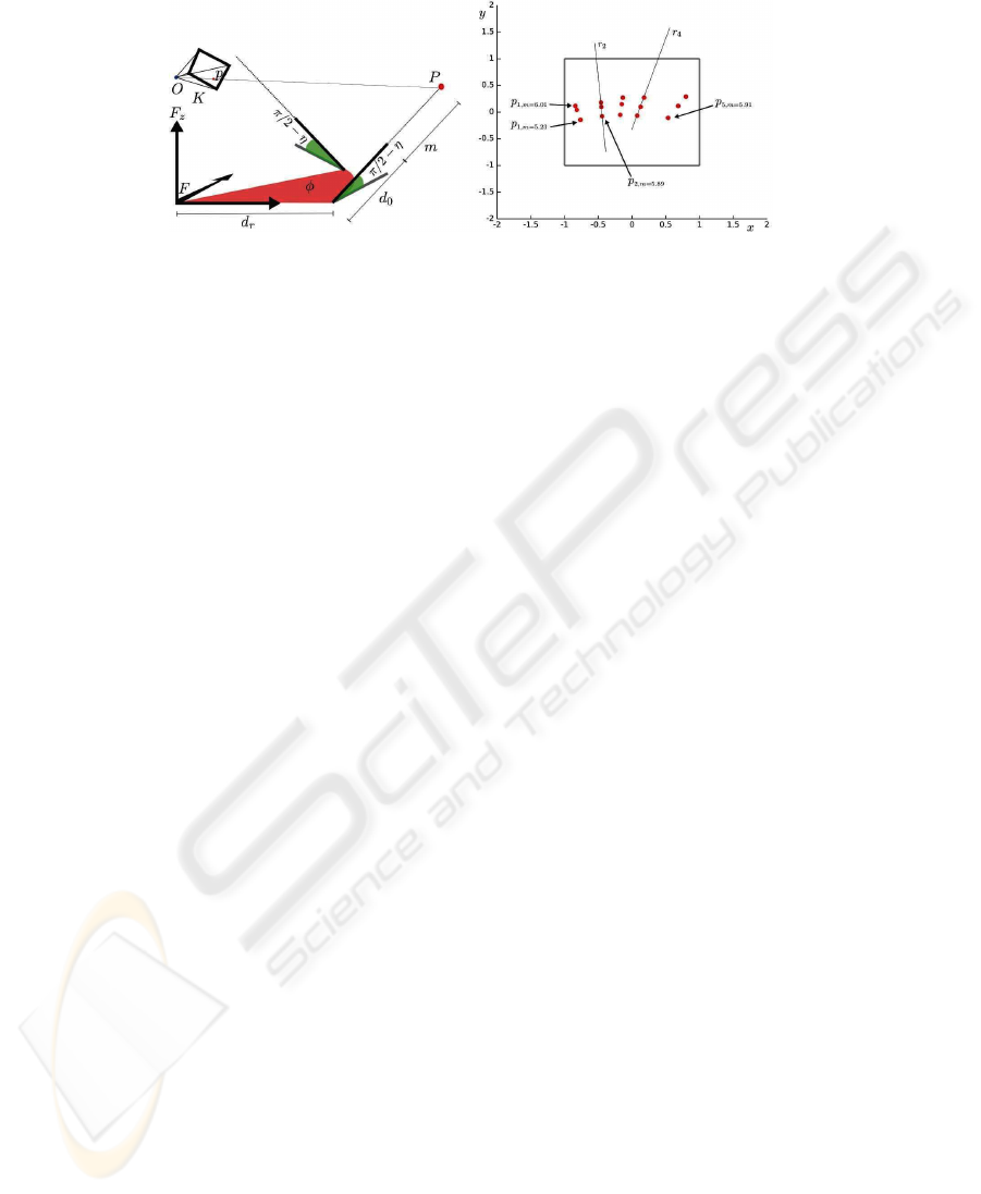
Fig. 1. Left: geometrical model of the system. Right: the minimal number of observations. For
each of the observed laser dots, the corresponding rangefinder measure is known. At least three
points are needed for each of 5 rangefinder angles.
2.2 System Parameters
Let r be a generic rangefinder ray; the rangefinder parameters are the following:
– the distance d
r
between r and F
z
;
– the angle η between r and F
z
;
– the distance d
0
between the point on r originating a zero rangefinder reading and
the point on r nearest to F
z
.
The camera parameters are expressed by the familiar perspective camera calibration
matrix P . More specifically, the intrinsic parameters are summarized by the K matrix,
on which we assume null skew factor, resulting in 4 degrees of freedom: aspect ratio a,
focal length f , and the principal point coordinates u
0
, v
0
. By considering 6 additional
degrees of freedom for the camera generic position and rotation w.r.t. F , the camera
model is characterized by 10 degrees of freedom.
In total, we are going to estimate a total of 13 system parameters.
2.3 Observation Model
The calibration procedure is based on a set of observations. Each observation o is char-
acterized by:
– a rangefinder rotation angle φ, not necessarily calibrated but repeatable;
– a rangefinder reading m;
– an image point p = (u, v), where the laser dot is observed.
We assume that the rangefinder reading is linear w.r.t. the actual distance in the scene,
up to the constant additive factor modeled by the rangefinder parameter d
0
.
φ and m identify a point in space, therefore they uniquely define the image point p
through the camera calibration matrix P and the rangefinder parameters.
3535
3 Calibration Procedure
3.1 Data Gathering
Our calibration procedure uses at least 15 observations; in Section 4 we show how the
procedure is extended in order to take advantage of additional observations or parame-
ters known a priori.
We consider 5 different φ angles φ
i
i = 1..5. For each i, we need 3 observations
o
i,j
j = 1..3 characterized by different m values. These observations can be easily
automatically gathered by simply moving the camera-rangefinder system in an environ-
ment, or by moving large objects in front of the still system.
o
i,j
= {i, m
i,j
, p
i,j
} (1)
3.2 Recovering Images of Coaxial Circles
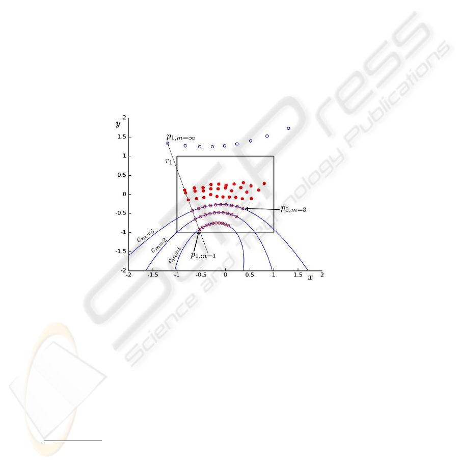
Fig. 2. Three conics can be recovered by exploiting the cross ratio invariance under perspective
transformations. Note that in this figure, observations for more than 5 angles are depicted.
p
i,1
, p
i,2
, p
i,3
are image points all lying on the same image line r
i
because they
are projections of scene points P
i,1
, P
i,2
, P
i,3
(the laser dots) lying on the same scene
line, i.e. the rangefinder ray R
i
1
. The distances between scene points P
i,1..3
are known
from the respective rangefinder readings m
i,1..3
: therefore, by exploiting the cross ra-
tio invariance under a perspective transformation, any point on image line r
i
can be
associated to the related rangefinder reading.
Let p
i,m=x
be the image point projection of the laser dot associated to rangefinder
reading x. We can now retrieve p
i,m=x
for any x. Then we compute p
i,m=1
, p
i,m=2
and
p
i,m=3
.
1
Even if the camera-rangefinder system is moved for gathering the observations, we are cur-
rently considering reference frame F , which is solidal with the system itself
3636
The procedure can be repeated for all of the 5 angles φ
i
i = 1..5. As a result, we get
another set of 15 points, corresponding to the projections of the laser dots associated to
the rangefinder readings m = 1, m = 2 and m = 3 for each of the 5 φ
i
angles. Note
that some of these image points may lie outside the imaged part of the image plane.
The 5 image points p
i,m=x
(with i = 1..5) all lie on a conic c
m=x
, because they
are projections of scene points lying on a circumference C
m=x
in the scene. The axis
of C
m=x
is the rangefinder rotation axis F
z
. We can reconstruct c
m=1
, c
m=2
and c
m=3
as we have 5 points belonging to each.
3.3 Computing the Camera Intrinsic Parameters
The images c
m=1
, c
m=2
and c
m=3
of three coaxial circles allow to calibrate the camera
parameters, and to recover the camera position with respect to the rangefinder. The
first step is to exploit c
m=1
, c
m=2
and c
m=3
in order to identify some vanishing points
representing orthogonal directions; then, the intrinsic camera parameters are determined
by exploiting the image of the absolute conic. We now describe the procedure in grater
detail.
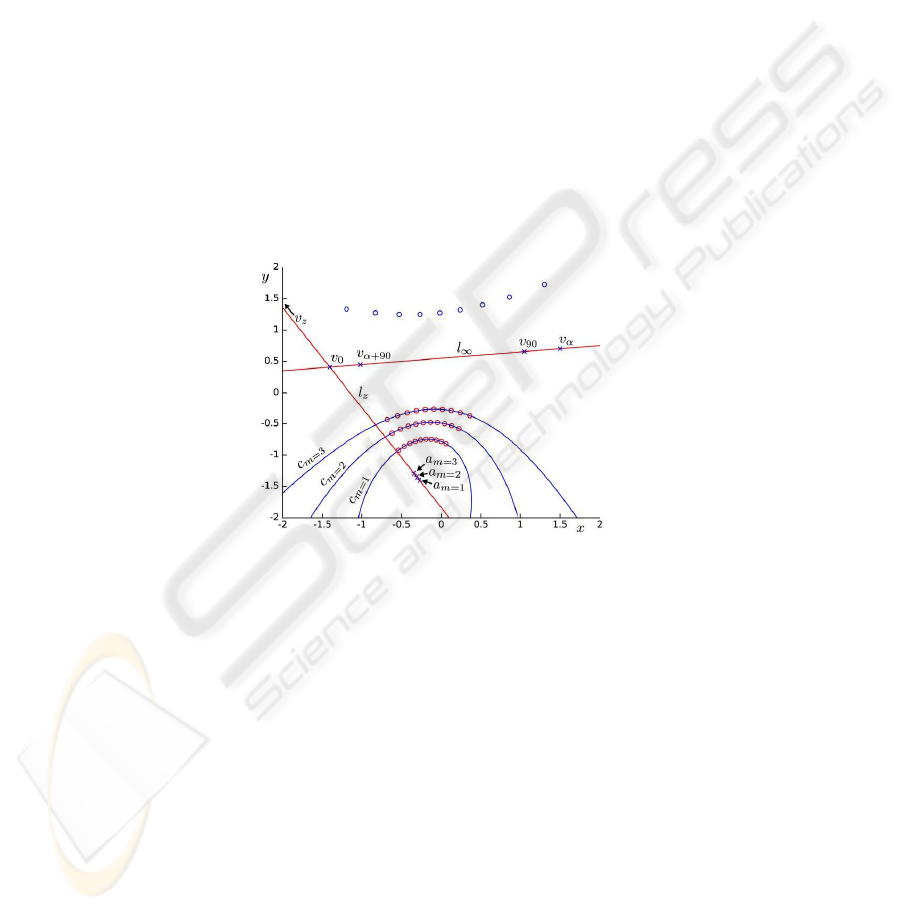
Fig. 3. The three conics allow us to derive a number of vanishing points, from which the camera
intrinsic parameters can be computed.
At first, we compute the intersection points of the three conics. The only two com-
mon intersection points are the projections of the two circular points of the xy plane;
they define the line at the infinity l
∞
of the xy plane in the image (horizon).
Let A
m=x
be the center of C
m=x
, and a
m=x
its projection. a
m=1
(a
m=2
, a
m=3
) is
easily found as the pole of l
∞
with respect to c
m=1
(c
m=2
, c
m=3
).
Let l
z
be the projection of the F
z
axis in the image. Since A
m=1
, A
m=2
and A
m=3
are aligned and lying on F
z
, l
z
is determined as the line passing through the a
m=x
points.
We name v
0
the intersection of l
z
with l
∞
, representing the horizontal vanishing
point associated to a direction belonging to the symmetry plane which is defined by
the camera center and rangefinder rotation axis. A vanishing point v
90
perpendicular to
such symmetry plane is found as the pole of l
z
with respect to any of the c
m=x
conics.
3737
Let v
α
be a different vanishing point randomly chosen on l
∞
; the vanishing point
v
α+90
is found as the intersection of l
∞
with the polar line of v
α
with respect to any of
the c
m=x
conics. v
α+90
represents a direction parallel to the xy plane and perpendicular
to the direction associated to v
α
.
Let v
z
be the vanishing point representing the F
z
direction. v
z
lies on l
z
; its exact
position can be recovered by considering points a
m=1
, a
m=2
and a
m=3
, which are
projections of equidistant points on F
z
; by means of the cross-ratio invariance, v
z
is
easily determined.
In order to find the camera intrinsic parameters, we exploit the image ω of the
absolute conic [5, 2]. ω can be recovered by exploiting orthogonality relations between
couples of the five vanishing points v
0
, v
9
0, v
α
, v
90+α
and v
α
, which translate to four
linear equations: v
T
α
ωv
α+90
= 0; v
T
z
ωv
0
= 0; v
T
0
ωv
90
= 0; and v
T
90
ωv
z
= 0
Once ω is known, the matrix K containing the camera intrinsic parameters can be
found using the Cholesky decomposition since ω = K
−T
K
−1
.
3.4 Recovering the Rangefinder Parameters
Computing η. The η angle between rangefinder rays and the rotation axis F
z
is eas-
ily recovered as the angle between the direction associated to a point p
i,m=∞
(which
represents a vanishing point of a rangefinder ray direction) and the direction associated
to v
z
; the angle between said directions can be computed since the camera intrinsic
parameters are now known.
p
i,m=∞
also allows us to recover the actual value of φ
i
, which was not previously
known: in fact, the projection of R
i
’s direction on the xy plane is identified by a van-
ishing point at the intersection between l
∞
and the join of p
i,m=∞
and v
z
; we can then
measure φ
i
in relation to the direction identified by v
0
.
The Radius of Circles C
m=x
. In order to recover the remaining rangefinder parame-
ters, we need to recover the radius of circles C
m=x
.
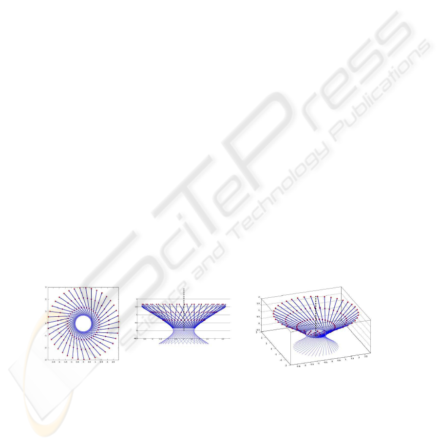
Fig. 4. The shape of the locus of rangefinder rays (a ruled quadric). The three circumferences
C
m=1
, C
m=2
and C
m=3
are shown. Note that their radius varies along the F
z
axis as an hyper-
bola.
We consider the two circles C
m=1
and C
m=2
, and the points P
1,m=1
, P
1,m=2
lying
on them, belonging to rangefinder ray R
1
. Let λ be the radius of C
m=1
: we are going to
3838

recover λ by writing an equation involving the length of the projection on the xy plane
of segment P
1,m=1
P
1,m=2
.
Let γ
m=1
be the (horizontal) direction of the radius A
m=1
P
1,m=1
. γ
m=1
is easily
recovered as the direction associated to the vanishing point found at the intersection
between l
∞
and the line on which said radius lies; the same holds for direction γ
m=2
of the radius A
m=2
P
1,m=2
.
Let κ be the ratio between radii κλ = A
m=2
P
1,m=2
and λ = A
m=1
P
1,m=1
. κ
can be recovered as follows: consider the image line bitangent to c
m=1
and c
m=2
at the
same side w.r.t. l
z
; let a
z
be the intersection point between said bitangent and l
z
, and A
z
its backprojection on F
z
. κ is now found as the ratio between the lengths of segments
A
z
A
m=2
and A
z
A
m=1
, which is computed exploiting the cross ratio invariance as:
κ = 2 ·
a
z
a
m=2
· a
m=0
a
m=1
a
z
a
m=1
· a
m=0
a
m=2
. (2)
We finally get a single equation in the single unknown λ, which leads to:
λ = cos(η)/
κ cos(γ
m=1
) − cos(γ
m=2
)
κ sin(γ
m=1
) − sin(γ
m=2
)
. (3)
Once λ is known, the radii of C
m=2
and C
m=3
are easily found.
Computing d
0
and d
r
. We can now consider the function y = f(x) relating a
rangefinder measure x to the radius of C
m=x
: it is a hyperbola with vertical axis, and
asymptotes forming an angle η with the x axis. Since we also have three points, we can
identify the hyperbola. Its vertex’ x and y coordinates are the rangefinder parameters
−d
0
and d
r
, respectively. Alternatively, d
r
can be recovered as the distance between the
3D line overlapping F
z
and the measuring ray which is easily identified by using the
data computed so far. d
0
immediately follows.
This concludes the calibration of the rangefinder parameters.
3.5 Recovering the Camera Position and Rotation
Recovering the camera position and rotation in the reference frame F is now possible.
The camera rotation matrix is easily computed from the location of vanishing points v
z
and v
0
. In order to compute the camera position, we can exploit the image of one of the
diameters of C
m=1
, whose 3D coordinates are now known.
4 Extensions, Discussion and Practical Issues
4.1 Degenerate Cases
If the camera center lies on the F
z
axis, the centers of all circumferences C
m=x
project
to the same image point; therefore, the presented technique does not apply.
Another degenerate case happens if η = 0 deg: then, the described procedure does
not allow the camera intrinsic parameters to be calibrated. Still, the first steps of our
3939

technique still allow us to recover a set of concentric, coplanar circles: by gathering
a first complete set of observations followed by another set acquired with a different
camera pose, the camera parameters can be calibrated and the rest of the procedure
follows with trivial modifications.
4.2 Exploiting Additional Observations
Since data gathering is such an easy and practical task, many additional observations
may be available in most scenarios with little additional effort. Our technique is easily
adapted to exploiting them, in order to improve the results accuracy and robustness to
noise.
For each of the φ
i
angles, we require at least three observations in order to recover
p
i,m=x
points by exploiting cross ratio invariance. If more than three different obser-
vations for a given φ
i
angle are available, the cross ratio can be estimated robustly to
noise. Note that measurement errors originate both from noise on the rangefinder read-
ings, and from uncertainty in the laser dot localization in the image.
If at least three observations are provided for more than five different φ angles, each
of the additional angles provides one extra point for estimating c
m=x
conics, which im-
proves noise resilience as well; then, known conic fitting techniques [3] can be applied.
Each of the p
i,m=x
points may be weighted differently, based on its confidence.
4.3 Exploiting a Priori Knowledge
In many scenarios, some of the system parameters may be known a priori; then, our
technique can be adapted in order to exploit this knowledge, in order to improve noise
resilience. Some common scenarios follow:
d
r
= 0 : in this case, the surface defined by the rangefinder rays is a cone: the last
part of the calibration can therefore be skipped; in fact, once λ is computed, d
0
is
immediately found.
Rangefinder parameters known: if all the rangefinder parameters are known a priori
and the φ angle of each observation is calibrated, rangefinder rays and laser dot
coordinates can be localized in reference frame F . Camera calibration then reduces
to the well-studied scenario in which all of the observed points have a known 3D
position.
Camera intrinsic parameters known : in this case, the first steps of the technique can
be skipped.
4.4 Visibility and Localization of the Laser Dot
Localizing the laser dot in an image is a task which is easily made automatic even in
lit environment: a simple solution, also suggested in [7] is shooting two images, one
with the laser on and one with the laser off; the difference image between the two then
isolates the laser dot, whose exact coordinates can be taken either by first binarizing the
image then using the skeletonize morphological operator, or by computing the barycen-
ter of the spot.
4040
In order to localize the dot, an obvious prerequisite is that it is actually visible in the
image: this may be a problem when using a laser working in the near-infrared wave-
lengths, whose dots will therefore irradiate light outside the visible part of the elec-
tromagnetic spectrum: although image sensors are very sensible to such wavelengths,
sometimes cameras use filters to minimize their effect, which should be removed.
5 Experimental Results and Implementation Notes
First, the technique has been validated by implementing a matlab-based simulator of the
camera-rangefinder system, also accounting for a customizable amount of normally-
distributed noise affecting both the image coordinates of the laser dot projection and
the readings of the rangefinder; we also developed a matlab implementation of the cali-
bration technique. When operating on clean data, the procedure yields results perfectly
adhering to ground truth (up to negligible errors due to numerical precision issues); this
validates the soundness of our approach. Figures 1 (right), 2 and 3 are related to such
experiments, with the following parameters: d
0
= 2, d
r
= 1, η = π/8, and a natural
camera with the principal point at the center of the image plane and focal length 0.55
times the image width. When adding noise, the quality of results drops rather dramat-
ically, due to the geometrical nature of the technique which is not resilient to noise.
In particular, intersecting conics returns unreliable circular points. Implementing the
techniques introduced in Section 4.2 allows to exploit additional observations, thus im-
proving noise resilience.
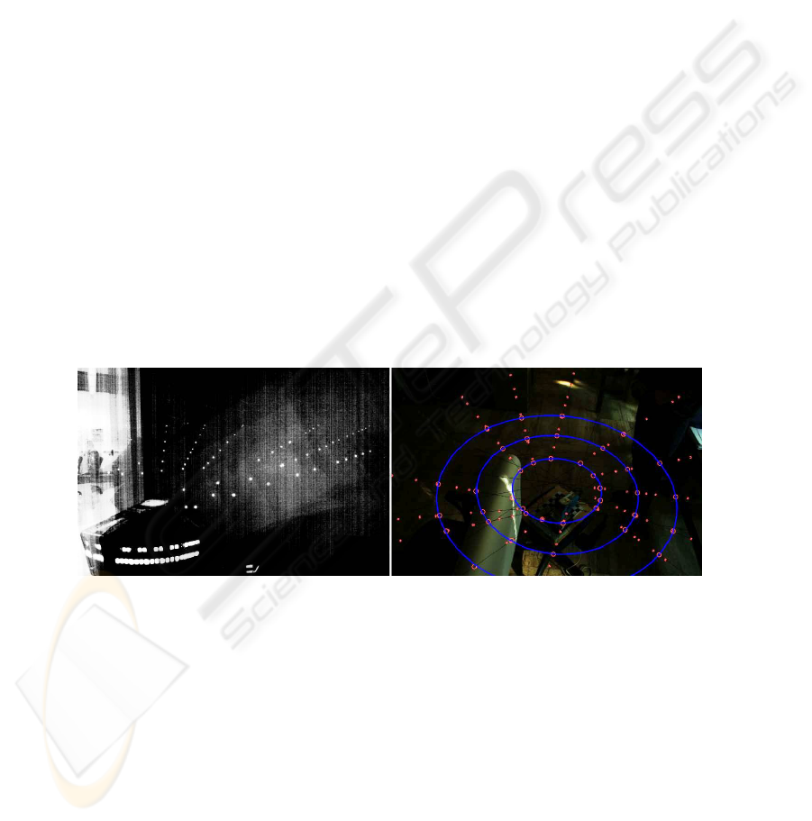
Fig. 5. Left: addition of many images shot in a dark room: the laser dots and their alignment are
visible; the dataset associates a range measurement with each. Right: part of the construction in
another real setting, on the background of one of the 92 images comprising the dataset; observa-
tions (red dots) and fitted lines (black); computed image points corresponding to 200mm, 400mm
and 600mm measures (red circles); fitted conics (blue ellipses); l
∞
is over the top of the image.
Note significant span of φ angles, which enables a much improved conic fitting.
We also applied the technique to camera images, acquired in two different sets with
different parameters, composed by 77 and 92 observations, respectively. Due to noise
in the image and rangefinder readings, all the observations must be exploited in order to
complete the calibration procedure correctly. However, we identified that some steps of
4141

the technique, such as the intersection of conics for finding l
∞
, are acting as bottlenecks
and being severely affected by noise. Such steps of the algorithm are currently being
improved and substituted with noise-resilient implementations in order to improve cal-
ibration accuracy in presence of noise.
6 Conclusions and Future Works
We developed a geometrical technique for mutually calibrating a camera and a laser
rangefinder. The technique is attractive because of its generality, and because it does
not assume anything about the environment; the data collection step is also extremely
simple and straightforward.
We validated the technique by using both real and simulated data: the results confirm
the correctness of the approach, but also highlight the expected weakness to noise in
the data when using the minimal amount of observations. In order to be practical in
real scenarios, we described a number of possible improvements aimed at increasing
robustness to noise; in particular, since data collection is fast and simple, the process
can be automated and may gather a large amount of observations.
We are currently implementing modifications to the technique in order to maxi-
mally exploit all available data, and replacing steps heavily affected by noise with noise-
resilient alternatives. Moreover, we are planning an extension for the mutual calibration
of a camera and a SICK laser rangefinder, whose scans are visible in the images as
jagged lines.
References
1. M. Antone and Y. Friedman. Fully automated laser range calibration. In Proc. of BMVC 2007.
2. Carlo Colombo, Dario Comanducci, and Alberto Del Bimbo. Camera calibration with two
arbitrary coaxial circles. In Proc. of ECCV 2006.
3. Andrew W. Fitzgibbon and Robert B. Fisher. A buyer’s guide to conic fitting. In Proceedings
of BMVC 1995.
4. Pierre Gurdjos, Peter Sturm, and Yihong Wu. Euclidean structure from n >= 2 parallel
circles: Theory and algorithms. In Proc. of ECCV 2006.
5. R. I. Hartley and A. Zisserman. Multiple View Geometry in Computer Vision. 2004.
6. G. Jiang, H. Tsui, L. Quan, and A. Zisserman. Geometry of single axis motions using conic
fitting. 2003.
7. C. Mei and P. Rives. Calibration between a central catadioptric camera and a laser range finder
for robotic applications. In Proc. of ICRA 2006.
8. Tom
´
a
ˇ
s Svoboda, Daniel Martinec, and Tom
´
a
ˇ
s Pajdla. A convenient multi-camera self-
calibration for virtual environments. PRESENCE: Teleoperators and Virtual Environments.
9. Qilong Zhang and R. Pless. Extrinsic calibration of a camera and laser range finder (improves
camera calibration). In Proc. of IROS 2004.
4242
