
Pose Clustering From Stereo Data
Ulrich Hillenbrand
Institute of Robotics and Mechatronics, German Aerospace Center (DLR)
82234 Wessling, Germany
Abstract. This article describes an algorithm for pose or motion estimation based
on clustering of parameters in the six-dimensional pose space. The parameter
samples are computed from data samples randomly drawn from stereo data points.
The estimator is global and robust, performing matches to parts of a scene with-
out prior pose information. It is general, in that it does not require any particular
object features. Empirical object models can be built largely automatically. An
implemented application from the service robotic domain and a quantitative per-
formance study on real data are presented.
1 Introduction
Estimation of the pose of known objects in unknown scenes is a basic problem within
many robotic applications. It arises not only in the context of object manipulation but
also of self localization and navigation in a known environment. Moreover, the prob-
lem of pose estimation is mathematically and algorithmically equivalent to the one of
motion estimation of objects or of the sensor itself relative to the environment. The
only difference between the two problems is that for pose estimation, one of the two
data sets that have to be registered is a priori known as the model of the object or the
environment.
Data acquired from a natural scene do not exclusively contain a single known ob-
ject, and two data sets in a motion sequence do not completely overlap. The estimator
hence needs to be robust in the statistical sense, that is, it must select in the estimation
process that part of the data that does match between two sets. Moreover, usually the
detailed correspondences, on the level of features or data points, even between the over-
lapping parts of two data sets, are not reliably known and must be established during
estimation. The combinatorics of the correspondence problem can give rise to a very
high proportion (approaching 100%) of effective outliers.
The estimation problem considered in this paper takes the correspondence and out-
lier problems to the extreme, in that i) no prior knowledge of object pose is assumed,
i.e., we aim at global pose estimation, and ii) no distinctive or high-level object features
are used, such that one is faced with a very large number of possible correspondences
between simple data points. Such simple data points can be, e.g., image points with
a gradient value above a threshold, edge and corner points [1], or range-data points
from stereo or laser imaging. The advantage of using simple data rather than distinctive
features is the general applicability to all kinds of objects and under a broad range of
imaging conditions. Distinctive features, on the other hand, require either the objects of
Hillenbrand U. (2008).
Pose Clustering From Stereo Data.
In VISAPP-Robotic Perception, pages 23-32
DOI: 10.5220/0002341900230032
Copyright
c
SciTePress

interest to possess certain characteristics (sharp edges, corners, colors, etc.) or that the
imaging conditions (viewpoint, lighting) do not significantly change (appearance-based
features, SIFT [2] and its variants).
There are various ways in which the present estimation algorithm relates to methods
used previously in pattern recognition. In fact, it may be understood as
– a continuous version of a randomized, generalized Hough transform,
– a density estimator in parameter space,
– a clustering procedure for parameter hypotheses.
Like parameter clustering in general, the method is based upon robust statistics in pa-
rameter space [3–8], as opposed to methods that rely on statistics in data space [9]. The
technique belongs to the class of non-parametric estimators, as no parametric models
of the underlying probability densities are assumed.
In the following section, the algorithm is described in some detail. The section on
experiments gives an example application to object manipulation that regularly runs in
our lab and a quantitative analysis of its performance on stereo data.
2 The Algorithm
The algorithm discussed in this paper is based upon range data. Other algorithmic vari-
ants of the same principle of pose clustering may process other types of data. The range
data is here obtained from a stereo algorithm that computes local correspondences in
an image pair from five partly overlapping correlation windows [10]. The outcome of
stereo processing is a point cloud with data points largely restricted to surface creases,
sharp bends, and depth discontinuities. Typical artifacts from correlation-based stereo
processing are also present, such as blurring of depth discontinuities and unstable depth
values for edges nearly parallel to the epipolar lines; see figs. 2 and 3.
The algorithm for object detection and pose estimation may be described as a se-
quence of three distinct steps:
1. model generation,
2. parameter sampling,
3. parameter clustering.
Model generation is an empirical process that runs offline and may hence be regarded as
a training step for the algorithm. Sampling and clustering of parameters are the actual
processing steps for scene data that need to run in real time. This section describes each
of these three steps in turn.
2.1 Model Generation
In a training phase, data of the sought objects are collected by the same sensing pro-
cess that is used later for recognition. In the present case, we collect range data points
produced by the stereo algorithm. Depending on the object’s complexity, between two
and, say, ten different views of the object are acquired. Different views are registered in
2424

an object coordinate system by an external pose measurement device, e.g., a robot. Al-
ternatively, given sufficient overlap between the data sets, a registration of the different
views may be achieved by the very same algorithm used later for pose estimation.
Data from different views are fused by discarding all points that are not stable under
view variation. More precisely, an intersection is computed of each data set in turn with
all the remaining data, allowing for a tolerance of a few millimeters for two data points
to be considered the same. These intersection sets are collected into the final data set.
Formally, given data sets D
1
, D
2
, . . . , D
n
acquired from different object views, the
model point set M is constructed as
M = ∪
n
i=1
D
i
∩
∪
n
j=1
j6=i
D
j
= ∪
n
i,j=1
i6=j
D
i
∩ D
j
, (1)
where the intersection tolerates small point differences. This procedure effectively re-
moves view-dependent artifacts of the sensing process, creating an idealized data point
set of the object. The point set M along with the lines of sight for each point consti-
tute the object model to be matched against scene data. The object model can be built
largely automatically with a robot that moves the sensor on the viewing sphere around
the object of interest.
2.2 Parameter Sampling
In order to produce a number of pose hypotheses, data samples are drawn from a scene
point set S and a model point set M from which pose parameter samples are com-
puted. A pose hypothesis can be computed from a minimum subset of three scene points
matched against a subset of three model points. The sampling proceeds thus as follows.
1. Randomly draw a point triple from S.
2. Randomly draw a point triple from M among all triples that are consistent with the
triple drawn from S.
3. Compute the rigid motion between the two triples in a least-squares sense.
4. Compute the six parameters of the hypothetical motion.
The parameter samples thus obtained are collected into a spatial array or a tree of buck-
ets, from where they can be efficiently retrieved for the subsequent clustering step. The
sampling process stops as soon as a significant number of parameter samples has accu-
mulated anywhere in parameter space. This condition is pragmatically taken as fulfilled
when one of the buckets is full. In numbers, from stereo data sets with 10
4
to 10
5
points
on the order of 10
6
point triples are drawn.
Corresponding data points from M and S can be found among geometrically con-
sistent groups of points. For drawing consistent point triples in sampling step 2, one
has to exploit the constraints that arise from rigid motion. These are i) approximate
congruence of the triangles defined by the point triples and ii) view point consistency.
The latter means that the plane defined by three simultaneously visible points on a non-
transparent solid shape generally exposes the same side to the sensor. Exceptions may
occur, e.g., for triples that span holes through a shape. Although the view point con-
straint does not hold for all points on all shapes under arbitrary motion, it is a useful
criterion for guiding the sampling process.
2525

The constraints are enforced by building a hash table of point triples from the model
M, which may in fact be done offline as part of the model generation process. The table
is accessed through a key that encodes a triple’s geometry in relation to the sensor.
Given three range data points r
1
, r
2
, r
3
∈ R
3
and their lines of sight l
1
, l
2
, l
3
∈ R
3
, a
suitable key (k
1
, k
2
, k
3
) ∈ R
3
is
k
1
k
2
k
3
=
||r
2
− r
3
||
||r
3
− r
1
||
||r
1
− r
2
||
if
(r
2
− r
1
) × (r
3
− r
1
)
T
(l
1
+ l
2
+ l
3
) > 0 ,
||r
2
− r
3
||
||r
1
− r
2
||
||r
3
− r
1
||
else,
(2)
where ||·|| denotes the Euclidean norm. When building the hash table, each model point
triple is entered for the key (k
1
, k
2
, k
3
) and its cyclic permutations (k
2
, k
3
, k
1
), (k
3
, k
1
, k
2
);
when sampling from the scene data, just one of the permutations is used for indexing
into the hash table. Through the hashing procedure, consistent scene-model pairs of
point triples can be efficiently drawn.
In step 3 of the sampling procedure, the least-squares rotation R
∗
∈ SO(3) and
translation t
∗
∈ R
3
between two point triples r
1
, r
2
, r
3
∈ M and r
0
1
, r
0
2
, r
0
3
∈ S are
computed, i.e.,
(R
∗
, t
∗
) = arg min
(R,t)∈SE(3)
3
X
i=1
||R r
i
+ t − r
0
i
||
2
. (3)
The method in [11] provides a solution, based on quaternions, that is specifically tai-
lored to the three-point case and hence more efficient than the general ones, like the
popular method based on singular value decomposition. If the three point pairs (r
i
, r
0
i
)
are approximately corresponding between M and S, the motion hypothesis (R
∗
, t
∗
)
will be close to the true object pose.
The choice of parameterization of motions in sampling step 4 is relevant for the
clustering of motion hypotheses. Indeed, the result of clustering depends upon the pa-
rameter space used. A proper choice is one that respects the topology of the Euclidean
group SE(3) [8]. Let α ∈ R
3
be the exponential/canonical parameters of the rota-
tion R
∗
, that is, ||α|| is the angle and α/||α|| the oriented axis of R
∗
. The parameters
ρ ∈ R
3
of rotations used here are related to the canonical parameters through
ρ =
||α|| − sin ||α||
π
1/3
α
||α||
, (4)
that is, a non-linear re-mapping of the rotation angle. Its desirable properties derive
from the fact that the invariant Haar measure of the rotation group SO(3) is uniform
in the parameters ρ, such that there is no bias of pose clustering incurred from the
group topology. This kind of parameterization has therefore been called consistent [8].
Translations are consistently parameterized simply by their three vector components
τ = t
∗
.
2626

2.3 Parameter Clustering
Significant populations of scene points in S matching a rigid motion of the model points
M will produce many parameter samples p = (ρ, τ ) ∈ R
6
that coincide approxi-
mately. The goal of parameter clustering is hence to estimate the location in parameter
space of the maximum probability density underlying the obtained parameter samples
{p
1
, p
2
, . . . , p
N
} [8]. A practical realization, derived from kernel density estimation, is
through the mean-shift procedure [12]. More precisely, a sequence of pose parameters
p
1
, p
2
, . . . is obtained through iterative weighted averaging
p
k
=
P
N
i=1
w
k
i
p
i
P
N
i=1
w
k
i
, (5)
w
k
i
= u
||ρ
k−1
− ρ
i
||/r
rot
u
||τ
k−1
− τ
i
||/r
trans
. (6)
Here u is a unit step function,
u(x) =
1 if x < 1,
0 else,
(7)
such that the averaging procedure (5) operates just on a neighborhood of p
k−1
. The
required parameter samples can be efficiently retrieved from buckets indexed by p
k−1
;
cf. sec. 2.2. The radii r
rot
and r
trans
of the rotational and translational extensions, re-
spectively, of the averaging procedure can be adapted to the local parameter density: a
higher density affords smaller radii.
The sequence p
k
converges to an estimate of the position of a local density max-
imum [12], even though the density of parameters is not explicitely estimated. By
starting with p
0
close to the dominant mode of the density, the sought pose estimate
ˆ
p = lim
k→∞
p
k
is thus obtained. The region of the dominant mode, in turn, is es-
timated from a histogram of pose parameters. Further modes may be explored in an
analogous fashion in order to identify additional object instances.
3 Experiments
3.1 An Application Scenario
The algorithm has been integrated into a humanoid robot system [13] which is used for
studying bi-manual manipulation. In particular, scenes composed of carafes, bottles,
jars, and glasses are visually analyzed to autonomously perform a sequence of actions
such as preparing a drink; see fig. 1. This kind of demonstration runs regularly in our
lab.
Figure 2 shows a typical scene as viewed through one of the head-mounted stereo
cameras and the stereo data with the recognized objects. Pose estimation is performed
on the complete data set, that is, without prior segmentation into the three object com-
ponents and the table component. The transparent objects are an example where reliable
extraction of more distinctive features than the raw stereo data can be a severe problem.
2727
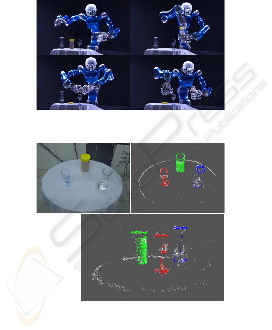
Fig. 1. DLR’s humanoid robot ‘Justin’ (upper body only) preparing a drink: after recognition of
the scene unscrewing the lid from a jar of instant tea, dropping some grains of tea into a glass,
and adding water from a carafe.
Camera image Data frontal view
Data side view
Fig. 2. Scene with objects used by the humanoid ‘Justin’ (cf. fig. 1) for preparing an instant-
tea drink: camera image and stereo data points (white) superposed with model points of the
recognized objects (colored).
2828
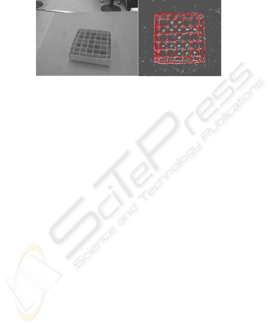
Data top viewCamera image
Fig. 3. Scene with a cardboard grid box used for quantitative evaluation of pose estimation ac-
curacy: camera image and stereo data points (white) superposed with model points of the box
(red).
3.2 A Quantitative Study
A quantitative analysis of pose estimation accuracy was carried out for a cardboard grid
box (approximate dimensions: 170 × 170 × 50 mm) that can contain metal pieces; see
fig. 3. For model building, an empty box was used. As test scenes, stereo data of the
partially filled box from 10 different views were acquired, while a robot moved the
stereo cameras around. Using the known motion of the robot between views, all the
data sets were registered in a common coordinate system. As a result, the pose that had
to be estimated was numerically the same for all sets.
However, a ground truth for the box pose was not available, both for practical and
for principle reasons. Practically, it is hard to rely on any other pose measurement to
be significantly more accurate than the one we want to test such that it could define the
reference pose. Moreover, in principle it is hard to define a true pose for a deformable
object such as the cardboard box, as in any setting it will slightly differ in shape from
the empty box seen at modeling time.
Avoiding these problems, two kinds of error statistics are here presented. One uses
the median of all pose estimates as the reference pose p
ref
to estimate the expected error
E(||
ˆ
p − p
ref
||). The other is based on the covariance matrix
C = E
n
[
ˆ
p − E(
ˆ
p)] [
ˆ
p − E(
ˆ
p)]
T
o
(8)
and estimates the square root of the total variation Tr C, which is a lower bound on the
expected quadratic error
E(||
ˆ
p − p
true
||
2
) = E[||
ˆ
p − E(
ˆ
p)||
2
] + ||E(
ˆ
p) − p
true
||
2
≥
E[||
ˆ
p − E(
ˆ
p)||
2
] = E{Tr [
ˆ
p − E(
ˆ
p)] [
ˆ
p − E(
ˆ
p)]
T
} = Tr C . (9)
Here p
true
is the true pose parameter and the neglected term ||E(
ˆ
p) − p
true
||
2
is the
squared bias of the estimator. Both error statistics are computed for the rotational and
translational parameters separately, because of their different physical dimensions.
2929

Pose estimates were computed either in a single stage or in two stages: the first stage
estimated the box rotation and translation in their joint 6D parameter space; an optional
second stage attempted to refine the translation estimate in its 3D parameter space while
keeping the estimated rotation fixed. Different resolutions of parameter space analysis
were investigated: the sizes of parameter buckets, histogram bins, and mean-shift radii
took identical rotational values {0.02, 0.03, 0.04, 0.05}
1
with their translational value
fixed at 30 mm for the first stage of estimation, and with identical translational values
{5, 10, 15} mm for the second stage. Estimator variants with only the first stage and
with both stages were run on the test data, making a total of 16 tested variants. Run
times of the estimators were recorded for a C++ implementation on a single CPU at 3.0
GHz. The measured times included building of the model hash table.
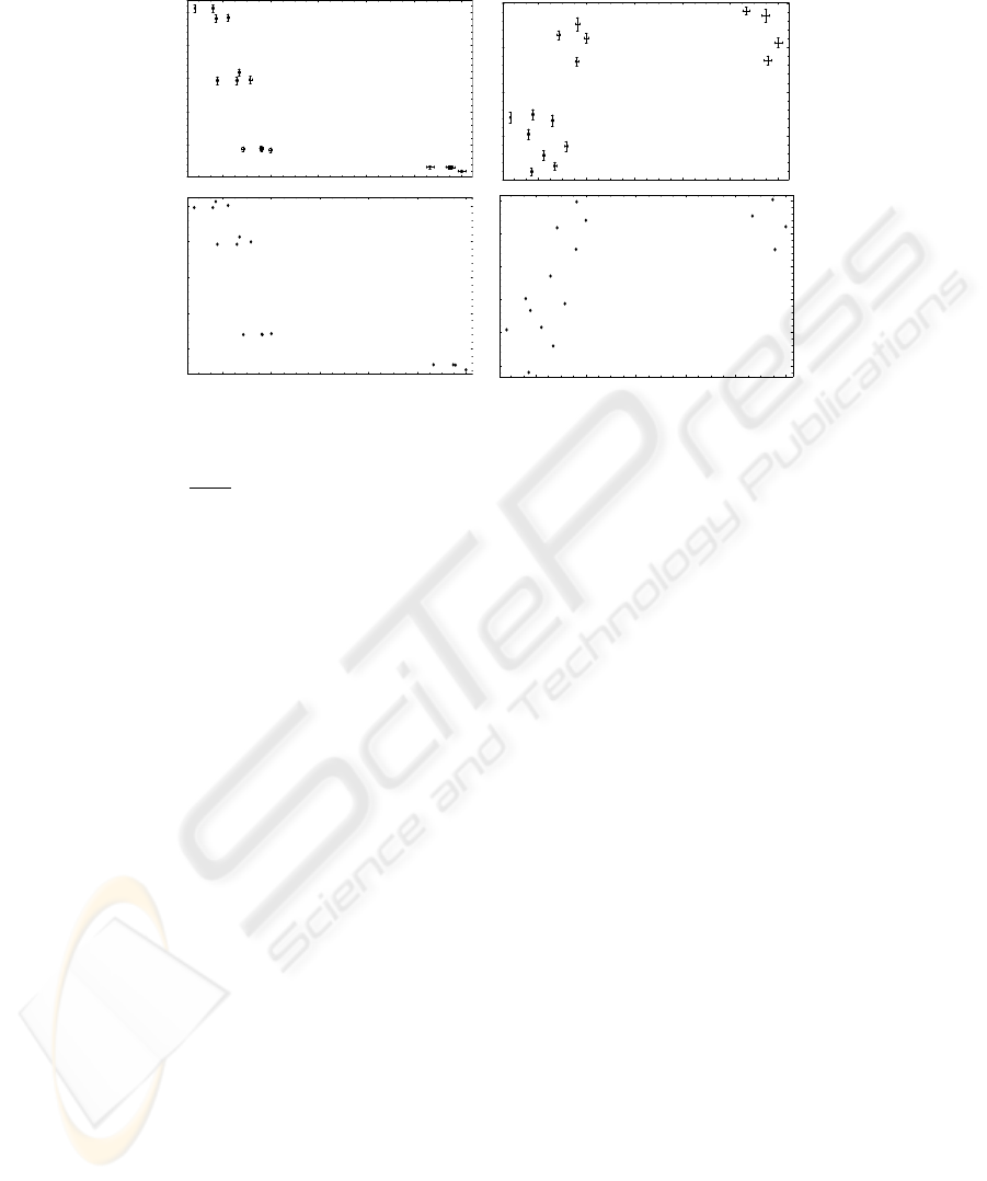
For each of the 10 box views, 100 data sets were acquired, yielding a total of 1000
pose estimates. Plots of the two kinds of error statistics, each for rotation and translation
estimates, versus expected run time for the 16 estimator variants are presented in fig. 4.
There are five main observations to be noted.
– The two kinds of error statistics agree, suggesting they are both reasonable error
measures for the estimates.
– The accuracy of the estimator is sufficient for manipulation tasks across all tested
variants.
– There is a trade off between rotational and translational accuracy.
– The highest rotational accuracy was achieved by estimators with the highest rota-
tional resolution; the highest translational accuracy was achieved by the estimator
with the lowest rotational resolution and the medium translational resolution in the
second estimation stage.
– The run time increases for estimator variants with higher resolution of parameter
space analysis; rotational resolution is much more expensive than translational res-
olution.
The last observation can be explained by the fact that smaller buckets in parameter
space need more sampling in order to get significantly filled. Sampling of full pose
parameters is much more expensive than of just translations, as done in the second
stage of estimation, which is why the translational resolution has less effect on run time
than the rotational resolution in the present statistics.
A less intuitive result is the apparent trade off between rotational and translational
accuracy. This suggests that, for the range of estimator variants here investigated, the
allover estimation error does not greatly vary but is merely distributed to varying pro-
portions between the rotational and translational degrees of freedom. As a consequence,
one should use different variants of the estimator for rotational and translational param-
eters. This point, however, deserves further investigation.
It should be noted that the run times given are mainly a relative measure of the costs
of the estimator variants. The absolute timings can be greatly improved by i) distribut-
ing parameter sampling and clustering across several CPUs, ii) building the model hash
tables before execution of the estimators, and iii) some additional algorithmic optimiza-
tions.
1
The full rotational parameter range is the unit sphere; cf. eq. (4).
3030
6 8 10 12 14 16
0.02
0.025
0.03
0.035
0.04
6 8 10 12 14 16
2.5
3
3.5
4
4.5
5
6 8 10 12 14 16
3.5
4
4.5
5
6 8 10 12 14 16
0.02
0.025
0.03
0.035
0.04
Total deviation [mm]
Total deviation [rad] Expected error [rad]
Expected error [mm]
Rotation Translation
Expected run time [s] Expected run time [s]
Fig. 4. Plots of error statistics versus run time statistics for the 16 tested variants of pose estimator:
expected error E(||
ˆ
p − p
ref
||) (bars indicate standard errors of the expectation values) and total
deviation
√
Tr C, each for rotation and translation parameters.
Acknowledgements
I greatfully acknowledge help with acquiring the test data from Michael Suppa and
Stefan Fuchs.
References
1. Harris, C., Stephens, M., A combined corner and edge detector. In: Fourth Alvey Vision
Conference. (1988) 147–151
2. Lowe, D.G., Distinctive image features from scale-invariant keypoints. Intern. J. Comput.
Vision 60 (2004) 91–110
3. Ballard, D.H., Generalizing the Hough transform to detect arbitrary shapes. Pattern Recog-
nition 13 (1981) 111–122
4. Stockmann, G., Kopstein, S., Benett, S., Matching images to models for registration and
object detection via clustering. IEEE Trans. Pattern Anal. Mach. Intell. 4 (1982) 229–241
5. Stockmann, G., Object recognition and localization via pose clustering. CVGIP 40 (1987)
361–387
6. Illingworth, J., Kittler, J., A survey of the Hough transform. CVGIP 44 (1988) 87–116
7. Moss, S., Wilson, R.C., Hancock, E.R., A mixture model for pose clustering. Patt. Recogn.
Let. 20 (1999) 1093–1101
8. Hillenbrand, U., Consistent parameter clustering: definition and analysis. Pattern Recogn.
Let. 28 (2007) 1112–1122
9. Stewart, C.V., Robust parameter estimation in computer vision. SIAM Review 41 (1999)
513–537
3131

10. Hirschm
¨
uller, H., Innocent, P.R., Garibaldi, J., Real-time correlation-based stereo vision with
reduced border errors. Int. J. Computer Vision 47 (2002) 229–246
11. Horn, B.K.P., Closed-form solution of absolute orientation using unit quaternions. J. Opt.
Soc. Am. A 4 (1987) 629–642
12. Comaniciu, D., Meer, P., Mean shift: a robust approach toward feature space analysis. IEEE
Trans. Pattern Anal. Mach. Intell. 24 (2002) 603–619
13. Ott, C., Eiberger, O., Friedl, W., B
¨
auml, B., Hillenbrand, U., Borst, C., Albu-Sch
¨
affer, A.,
Brunner, B., Hirschm
¨
uller, H., Kielh
¨
ofer, S., Konietschke, R., Suppa, M., Wimb
¨
ock, T.,
Zacharias, F., Hirzinger, G., A humanoid two-arm system for dexterous manipulation. In:
Proc. IEEE-RAS International Conference on Humanoid Robots. (2006) 276–283
3232
