
MAPPING LANDMARKS ON TO THE FACE
G. M. Beumer, R. N. J. Veldhuis and B. J. Boom
Signals and Systems Group, University of Twente, P.O. Box 217 7500 AE, Enschede, The Netherlands
Keywords:
Landmarking, Face recognition, Biometrics.
Abstract:
Landmarking can be formalised as calculating the Maximum A-posteriori Probability (MAP) of a set of land-
marks given an image (texture) containing a face. In this paper a likelihood-ratio based landmarking method
is extended to a MAP-based landmarking method. The approach is validated by means of experiments. The
MAP approach turns out to be advantageous, particularly for low quality images, in which case the landmark-
ing accuracy improves significantly.
1 INTRODUCTION
An important prerequisite for reliable face recogni-
tion is that the face is registered prior to recognition.
Registration is the alignment of the face to a fixed
position, scale and orientation. Registration in face
recognition is usually based on landmarks, which are
stable points in the face that can be found with suffi-
cient accuracy, e.g. the eyes. A reliable method for
automatic landmarking and registration is essential
for the automatic face recognition. The accuracy of
the landmarking has been shown to have a strong re-
lation to the recognition result (Beumer et al., 2005).
Work on landmarking includes, amongst others,
(Everingham and Zisserman, 2006), in which the
authors compare a regression method, a Bayesian
method, and finally a discriminative method for land-
marking. Work by (Cristinacce and Cootes, 2006) fo-
cuses on both multiple templates of the landmark and
the landmark coordinates to constrain the search area.
The above approaches do not explicitly use the proba-
bility of the landmark coordinates. In this paper these
will be exploited by extending a method based on a
log likelihood ratio to a Maximum A-posteriori Prob-
ability (MAP) approach (van Trees, 1968).
In (Bazen et al., 2003) image data at each posi-
tion in a region of interest is compared to a landmark
template by a log-likelihood ratio based detector. The
position at which the log-likelihood ratio is highest
is taken as the position of the landmark. This ap-
proach has been further developed to the Maximally
Likely Landmark Locator (MLLL) and extended with
a subspace-based outlier-correction method called
BILBO in (Beumer et al., 2006).
The maximization of the likelihood ratio is a
heuristic approach, not necessarily leading to the best
position for the landmark. Note that any position
characterized by a likelihood ratio above a pre-set
threshold can be a landmark with certain probabili-
ties of false acceptance and false rejection, dependent
on the threshold. Therefore, we will reformulate the
likelihood-ratio based methods in (Bazen et al., 2003)
and (Beumer et al., 2006) to a MAP approach, thus
giving it a solid theoretical foundation, taking the a-
priori probability of a landmark location into account.
This will prove to make the method robust against
outliers. In a first attempt to validate this approach we
performed a simple experiment. Its results show that
the new method performs significantly better than the
likelihood-ratio based methods, in particular on low
quality images.
2 THEORY
The shape
~
s of a face is defined as the collection of
landmark coordinates, arranged into a column vector.
The landmark coordinates belong to a facial area with
texture ~x, measured in a certain region of interest and
also arranged into a column vector. The MAP esti-
mate,
~
s
∗
, given a certain texture ~x, can be written as
~
s
∗
= argmax
~
s
q(
~
s|~x) (1)
According to Bayes rule, Equation 1 can be written as
~
s
∗
= argmax
~
s
p(~x|
~
s)
p(~x)
q(
~
s), (2)
12
Beumer G., Veldhuis R. and Boom B. (2009).
MAPPING LANDMARKS ON TO THE FACE.
In Proceedings of the International Conference on Bio-inspired Systems and Signal Processing, pages 12-17
DOI: 10.5220/0001431100120017
Copyright
c
SciTePress
where p(~x|
~
s) is the probability of the texture ~x given a
landmark location; p(~x) is the background probabil-
ity; and q(
~
s) is the probability of the shape as func-
tion of the location
~
s. The quotient Equation 2 is the
likelihood-ratio of the texture belonging to shape
~
s
over the overall texture probability. The last factor
takes the probability of the shape at location
~
s into
account. Ideally, one would like to compute
~
s from
Equation 2, given all probabilities. This, however
would be prohibitively complex. Therefore a number
of simplifications are introduced.
Let
~
s
i
∈ R
2
denote the column vector containing
the spatial coordinates of landmark i = 1...l and ~x
i
∈
R
n
the column vector containing the n pixel values
from the texture in a region of interest surrounding the
assumed landmark i. These landmarks are illustrated
in Figure 1.
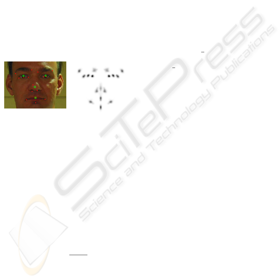
Figure 1: Left: the landmarks used from the BioID database
-dots- and from the FRGC -circles-. Right: The shape dis-
tributions map showing the 17 landmarks.
We assume that ~x
i
only depends on
~
s
i
and that ~x
i
and~x
j
, i 6= j, are independent. The latter is plausible if
there is no overlap between~x
i
and~x
j
. We also assume
that the landmarks locations are mutually indepen-
dent, though we know this assumption to be incorrect.
However, this assumption creates an easer framework
because then q(
~
s) can be written as
∏
q(
~
s
i
). In later
work this assumption will be dropped. The distri-
bution of the shapes q(
~
s
i
) is determined empirically
through histograms. This results in a two-dimensional
landscape for each landmark representing the proba-
bility distribution. The probability distributions q(
~
s
i
)
for a number of landmarks can be seen in Figure 1.
With these simplifications Equation 2 can be rewrit-
ten as:
~
s
∗
= argmax
~
s
l
∏
i=1
p(~x
i
|
~
s
i
)
p(~x
i
)
q(
~
s
i
) (3)
The quotients in the product are optimized by the
MLLL algorithm by (Beumer et al., 2006).
3 IMPLEMENTATION
Equation 3 can be rewritten as
~
s
∗
= argmax
~
s
l
∑
i=1
log(p(~x
i
|
~
s
i
)) −
log(p(~x
i
)) + log(q(
~
s
i
))
(4)
We assume that p(~x
i
|
~
s
i
) is Gaussian with mean µ
l,i
and covariance Σ
l,i
and, likewise, that p(~x
i
) is Gaus-
sian with mean µ
b,i
and covariance Σ
b,i
. Gaussian
mixture models might model the data better, but they
would also be much more complex. Because of the
assumed mutual independence of the landmarks, the
terms in Equation 3 can be maximized independently.
This makes that the estimation of the shape, for all
landmarks i = 1 . . .l, now is simplified to
~
s
∗
i
= argmax
~
s
−
1
2
(x
i
− µ
l,i
)
T
Σ
−1
l,i
(x
i
− µ
l,i
) +
1
2
(x
i
− µ
b,i
)
T
Σ
−1
b,i
(x
i
− µ
b,i
) +
log(q(
~
s))
(5)
for all landmarks i = 1 . . .l.
3.1 Dimensionality Reduction
Because ~x
i
consists of a large number of statistically
dependent pixels it is possible and useful to perform
a dimensionality reduction. The covariance matri-
ces, Σ
l
and Σ
b
, need to be estimated from training
data. Due to their size, direct evaluation of Equa-
tion 5 would be a high computational burden. Due
to the limited number of training samples available
in practice, they would be rank-deficient or, if not,
too inaccurate to obtain a reliable inverse, which is
needed in Equation 5. For example, a typical train-
ing image consists of between 1000 and 5000 pixels
while there are only 3042 (see Section 4) landmark
samples. Therefore, prior to evaluation of Equation 5,
the vector ~x will be projected onto a lower dimen-
sional subspace. This subspace should have several
properties. First of all, its basis should contain the
significant modes of variation of the landmark data.
Secondly, it should contain the significant modes of
variation of the background data. Finally, it should
contain the difference vector between the landmark
and the background means for good discrimination
between landmark and background data. The modes
of variation are found by principal component analy-
sis (PCA). See Appendix A for details.
Finally, the landmark and background densities
are simultaneously whitened such that the landmark
covariance matrix becomes a diagonal matrix, Λ
L
,
and the background covariance matrix becomes an
identity matrix.
MAPPING LANDMARKS ON TO THE FACE
13

3.2 Feature Extraction
and Classification
The entire process of dimensionality reduction and si-
multaneous whitening can be combined into one lin-
ear transformation with a matrix T
i
∈ R
n×m
, with n
the dimensionality of the training templates and m the
final number of features after reduction.
˜µ
l,i
= T
i
µ
l,i
, ˜µ
b,i
= T
i
µ
b,i
(6)
˜
Σ
l,i
= T
i
Σ
l,i
T
T
i
,
˜
Σ
b,i
= T
i
Σ
b,i
T
T
i
(7)
~y
i
(
~
s
i
) = T
i
~x(
~
s
i
) (8)
For the i-th landmark Equation 5 now becomes
~
s
∗
i
= argmax
~
s
−
1
2
(~y
i
(
~
s) − ˜µ
l,i
)
T
˜
Λ
−1
l,i
(~y
i
(
~
s) − ˜µ
l,i
)
+
1
2
(~y
i
(
~
s) − ˜µ
b,i
)
T
(~y
i
(
~
s) − ˜µ
b,i
)
+log(q(
~
s))
(9)
The feature vector,~y
i
(
~
s), at location
~
s for the i-th land-
mark is extracted from texture date in the region of
interest, ~x
(
~
s). The detailed calculation of the feature
reduction transformation T
i
is given in Appendix A.
Note that although Equation 9 resembles Equation 5,
the result will be different due to the dimensionality
reduction. This form is however computationally far
more efficient then Equation 5.
4 EXPERIMENTS
Two databases were used. The BioID database (Hu-
manScan, ) was used for training the algorithms, i.e.
estimating T
i
, ˜µ
l,i
, ˜µ
b,i
,
˜
Σ
l,i
and
˜
Σ
b,i
. The FRGC
database (Phillips et al., 2005) was used to test the
algorithms.
The BioID consists of 1521 images of 22 per-
sons. The BioID images have 20 labelled landmarks
of which 17 are used: the eye centres, inner and outer
eye corners, inner of outer ends of the eyebrows, both
nostrils, the tip of the nose, both mouth corners and
the centre of both the upper lip and the lower lip.
For each of these 17 landmarks a MAP classifier was
trained. From each image two positive samples were
taken for each landmark, both symmetrical and asym-
metrical. For all symmetrical landmarks a mirrored
version of the landmark has been added. Asymmet-
rical landmarks, such as the eyes, come in pairs. For
all asymmetrical landmarks a mirrored version of the
other has been added. For example a mirrored ver-
sion of the left eye was used as a right eye. For each
landmark this gives 3042 landmark samples.
The background samples are taken randomly and
uniformly from an area around the landmark location.
Around each landmark from each image ten negative
samples were taken. The minimal and maximal dis-
tance from the landmark location to the centre of the
background training image were fixed. The minimal
distance was 0.25 times the size of the training image.
The maximum distance was the width of the image it-
self. This is illustrated in Figure 2.
Figure 2: The rectangle landmark sample is shown as a solid
line. The + denotes the centre of the image. The grey area
shows the possible locations of the centre of the background
samples. Three possible background samples are shown by
dashed lines.
The FRGC 2.0 database consists of a controlled
set of images with high quality and an uncontrolled
set of images with low quality. Both sets will be used
separately in the experiment. In total the FRGC 2.0
database contains 39328 images, roughly one third
are low quality images and two third are high quality
images. The FRGC 2.0 images have ground truth co-
ordinates for the eyes, nose and mouth. A (Viola and
Jones, 2001) classifier from the OpenCV library (In-
tel, ) was used to locate the face in each image. The
algorithm was run on each face correctly found by the
Viola and Jones classifier (38829, 98.7% of all im-
ages). Since the algorithm always produces an esti-
mate, there are 38829 sets of coordinates to evaluate.
There is a difference between the ground truth co-
ordinates in the FRGC 2.0 database and the landmarks
in the BioID training data. Therefore, we converted
the landmarks found to FRGC ground truth. Several
of the coordinates found by the algorithms are aver-
aged into one compound coordinate, which is com-
pared to the ground truth data. In Table 1 an overview
is given.
Table 1: Overview of the compound coordinates.
FRGC Landmarks found and averaged
Eye Both eye corner and the eye centre.
Nose Tip of the nose and both nostrils.
Mouth Upper lip, lower lip and both mouth corners.
In order to evaluate the quality of the methods
used we used the same measure as in (Cristinacce and
BIOSIGNALS 2009 - International Conference on Bio-inspired Systems and Signal Processing
14
Cootes, 2006):
m
e
=
1
n∆
ocl
n
∑
i=1
q
δ
2
i,x
+ δ
2
i,y
(10)
where n is the number of landmarks, ∆
ocl
the inter oc-
ular distance in the ground truth data, δ
i,x
and δ
i,y
the
displacements of the i-th landmark. This number is
calculated for each image and each landmark. From
the error a bias had to be removed. This was to com-
pensate for offsets in the error due to compounding.
The average of the three points on the nose is not the
same as the tip of the nose. Also both databases could
be labelled differently, what in the BioID is consid-
ered the tip of the nose is not necessary what the mak-
ers of the FRGC 2.0 considered to be the tip of the
nose.
Both MAP and MLLL were run individually and
in combination with BILBO (Beumer et al., 2006).
Original versions of MLLL and BILBO were kindly
availed to us by the authors. All results were evalu-
ated and compared to each other.
5 RESULTS
Figure 1 shows an example of a set of found land-
marks. The red dots denote the estimated landmark
locations and the green circles show the ground truth
data. In Table 1 the relation between the 17 estimates
and the 4 ground truth labels is defined. Most land-
marks estimated were rather accurately and a few are
slightly off.
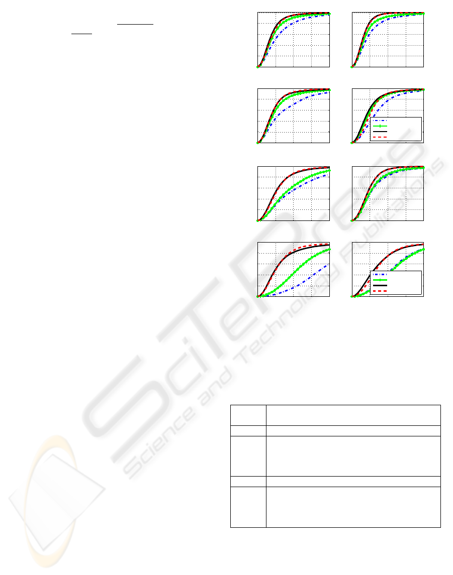
In Figure 3 the cumulative error plots are shown.
They are split into two sets. The top block of 4
plots shows the cumulative errors for the high qual-
ity images and the bottom block of 4 plots for the low
quality images. The upper right plot of each block
of 4 plots shows the overall error. The upper left
plot shows the error for the eyes. The bottom plots
show the graphs for the nose and mouth. In each plot
there are curves for MLLL, MLLL+BILBO, MAP
and MAP+BILBO.
The results are also shown in Table 2. This table
shows the average error for a certain landmark. In or-
der to compare the results, the average errors obtained
by MLLL and BILBO algorithms are also presented.
5.1 Discussion
The MAP method performs better than MLLL on
both the high quality images and the low quality im-
ages. Interestingly, the improvement on the low qual-
ity data is far greater than on the high quality data.
The robustness of the MAP approach is better than
0 5 10 15 20
0
20
40
60
80
100
Portion errors
Error in % of the interocular distance
High quality images − All
0 5 10 15 20
0
20
40
60
80
100
Portion errors
Error in % of the interocular distance
Eyes
0 5 10 15 20
0
20
40
60
80
100
Portion errors
Error in % of the interocular distance
Nose
0 5 10 15 20
0
20
40
60
80
100
Portion errors
Error in % of the interocular distance
Mouth
1−MLLL
2−MLLL+BILBO
3−MAP
4−MAP+BILBO
0 5 10 15 20
0
20
40
60
80
100
Portion errors
Error in % of the interocular distance
Low quality images − All
0 5 10 15 20
0
20
40
60
80
100
Portion errors
Error in % of the interocular distance
Eyes
0 5 10 15 20
0
20
40
60
80
100
Portion errors
Error in % of the interocular distance
Nose
0 5 10 15 20
0
20
40
60
80
100
Portion errors
Error in % of the interocular distance
Mouth
1−MLLL
2−MLLL+BILBO
3−MAP
4−MAP+BILBO
Figure 3: The cumulative error. Top rows: high quality
images. Bottom rows: low quality images.
Table 2: The average error for the three methods. Total
means the mean RMS error for all coordinates together. The
bracketed number gives the relative improvement of both
MAP and MAP+BILBO compared to MLLL+BILBO.
MLLL MLLL+ MAP MAP+
BILBO BILBO
High quality images
Total 6.8 5.2 4.3 (17%) 4.4 (15%)
Eye 5.7 4.6 3.4 (26%) 3.5 (24%)
Nose 8.2 5.8 4.9 (16%) 4.7 (19%)
Mouth 7.7 5.8 5.4 (7 %) 5.9 (-2%)
Low quality images
Total 11.3 9.6 6.3 (34%) 6.3 (34%)
Eye 6.8 6.5 5.1 (22%) 5.0 (23%)
Nose 18.9 12.6 7.2 (43%) 6.7 (47%)
Mouth 12.6 13.1 8.1 (38%) 8.4 (36%)
that of MLLL. For MAP the gap between the perfor-
mance on the high quality images and the low quality
images is significantly reduced compared to MLLL
and MLLL+BILBO. This can be attributed to the a
priori term q(
~
s). When the likelihood term is rather
flat as a function of
~
s, the influence of the q(
~
s) is
strongest. This seems to occur more often in the low
quality ies than in high quality images.
MAPPING LANDMARKS ON TO THE FACE
15
Region of intrest
−2
−1
0
A priori landscape
−30
−20
−10
Likelihood landscape
−100
−80
−60
−40
−20
MAP landscape
−150
−100
−50
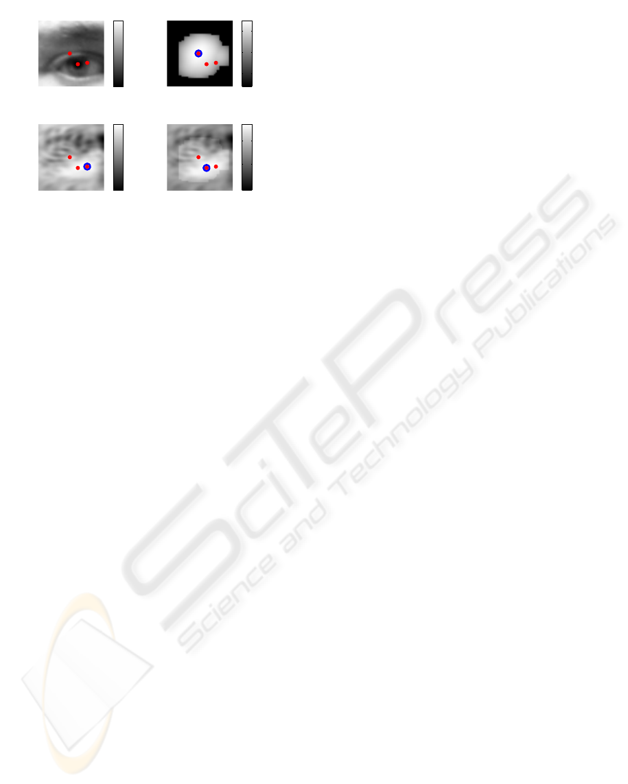
Figure 4: The top row shows an eye on the left and on
the right the a priori landscape is presented. The bottom
row presents the likelihood landscape on the left and finally
the MAP landscape. The blue circles denote the maximum
in that landscape while red dots are the landscape maxima,
shown for easy reference.
In Figure 4 a detailed example for one landmark,
an eye, can be seen. In the upper right corner we see
a region of interest for the eye. The upper right shows
the a priori landscape for this landmark. The lower
left corner shows the likelihood-ratio landscape. This
is the sum of the first two terms of Equation 9. Finally,
in the lower right corner the resulting MAP landscape
is shown. In each landscape the location of the max-
imum value is denoted by a large blue circle. In each
of the four images the maxima of the three landscapes
are plotted as a red dot for easy reference. The max-
ima of the likelihood ratio landscape and the MAP
landscape are shown as the two red dots. It can clearly
be seen that because of the influence of the q(
~
s) MAP
gives a better estimate of the centre of the eye. It is,
however, also true that the final influence of the q(
~
s)
term is not always as substantial as in Figure 4. MAP
improves the result here because the likelihood land-
scape is rather uniform in the entire eye region. It
is reasonably save to assume that a part of the im-
provement with regards to MLLL and BILBO can be
attributed to better implementation of the feature ex-
traction then the one in the original MLLL. If a likeli-
hood ratio landscape has a sharp maximum, as in high
quality images, there is not much contribution of the
shape probability to the final MAP landscape.
Finally, two interesting observations can be made.
First, applying BILBO is not always beneficial. Ap-
plying BILBO to the MLLL and MAP data makes in-
creases the error for the mouth except for MLLL in
the high quality images. This can be seen in both
Table 2 and Figure 3. Possible explanations for this
effect can be that landmark locations on the mouth
are falsely corrected by BILBO because of grand er-
rors on for instance the nose. Secondly, it is clear that
BILBO does not significantly improves MAP while
it does improve the results of the MLLL algorithm.
From this we can conclude that MAP has less severe
outliers and that the limit of BILBO is being reached.
Also, with MAP the shape is already taken into ac-
count more than with MLLL alone. On the other
hand, the fact that using a shape based outlier detec-
tion sometimes still improves the results proves that
there is still room for improvement of the current im-
plementation of the MAP algorithm.
5.1.1 Future Improvements
This method can be further improved by dropping
the assumption made in Section 3 that the landmarks
are independent. This requires a more elaborate op-
timization method for solving Equation 2. Also the
quality of the training data is not sufficient. The
BioID database only contains landmarks from 22 per-
sons. Training on a different database with a bigger
variety of persons might improve the results signifi-
cantly.
Further improvement can be reached by making
an iterative implementation of the algorithm. In the
current implementation, the algorithm trained solely
on registered images. The algorithm responds works
less good on unregistered faces. This has a twofold
negative effect. First the likelihood landscape is cal-
culated for a type of image it has not been trained
to recognize. Secondly the probability distribution of
the shape assumes the head to be aligned. When the
MAP algorithm is used iteratively, an image is better
aligned each run. Thus it has a better fit to the model,
improving the overall accuracy.
6 CONCLUSIONS
We formulated a solid MAP frame work for finding
the landmarks in a facial image. Our implementation,
however, is only a first step towards a complete MAP
landmark location estimator. It shows that using the
MAP probability actually improves the performance
of the MLLL and BILBO algorithms on frontal still
images. MAP has turned out to be more robust be-
cause the performance on the low quality images im-
proved a lot, narrowing the performance gap with the
high quality images. The assumption that we made
that the landmark locations are independent is incor-
rect. The next step will be to introduce the dependen-
cies between the landmarks in order to improve the
estimates of q(
~
s). Also making an iterative implemen-
tation can improve the MAP approach. Nevertheless
the results are promising.
BIOSIGNALS 2009 - International Conference on Bio-inspired Systems and Signal Processing
16

REFERENCES
Bazen, A. M., Veldhuis, R. N. J., and Croonen, G. H.
(2003). Likelihood ratio-based detection of facial fea-
tures. In Proc. ProRISC 2003, 14th Annual Workshop
on Circuits, Systems and Signal Processing, pages
323–329, Veldhoven, The Netherlands.
Beumer, G. M., M.Bazen, A., and Veldhuis, R. N. J. (2005).
On the accuracy of eers in face recognition and the
importance of reliable registration. In SPS 2005. IEEE
Benelux/DSP Valley.
Beumer, G. M., Tao, Q., Bazen, A. M., and Veldhuis, R.
N. J. (2006). A landmark paper in face recognition. In
Automatic Face and Gesture Recognition, 2006. FGR
2006. 7th International Conference on, Southampton,
UK, Los Alamitos. IEEE Computer Society Press.
Cristinacce, D. and Cootes, T. F. (2006). Facial feature
detection and tracking with automatic template se-
lection. In FGR ’06: Proceedings of the 7th Inter-
national Conference on Automatic Face and Gesture
Recognition (FGR06), pages 429–434, Washington,
DC, USA. IEEE Computer Society.
Everingham, M. and Zisserman, A. (2006). Regression and
classification approaches to eye localization in face
images. In FGR ’06: Proceedings of the 7th Inter-
national Conference on Automatic Face and Gesture
Recognition (FGR06), pages 441–448, Washington,
DC, USA. IEEE Computer Society.
HumanScan. Bioid face db. http://www.humanscan.de/.
Intel. Open computer vision library. http:// source-
forge.net/projects/opencvlibrary/.
Phillips, P. J., Flynn, P. J., Scruggs, T., Bowyer, K. W.,
Chang, J., Hoffman, K., Marques, J., Min, J., and
Worek, W. (2005). Overview of the face recognition
grand challenge. In In Proceedings of IEEE Confer-
ence on Computer Vision and Pattern Recognition.
van Trees, H. (1968). Detection, Estimation and Modula-
tion Theory, Part I. John Wiley and Sons, New York.
Viola, P. A. and Jones, M. J. (2001). Rapid object detection
using a boosted cascade of simple features. In CVPR
(1), pages 511–518.
APPENDIX
A Dimensionality Reduction
The subspace should contain a good representation of
the variations of both the landmark data, X
l
, and the
background data, X
b
. Each column of data matrices
X
l
and X
b
is a single training sample x
s
. Therefore,
two projections matrices U
l
and U
b
follow from the
singular value decomposition (SVD)
U
(l,b)
S
l,b
V
T
l,b
= (X
l,b
− M
l,b
), (11)
where M
l,b
= µ
l,b
[1. . . 1], i.e. a matrix whose
columns are the column average of X. For reasons
of computational complexity we only keep the first
columns of U
l
and U
b
, which represent a fixed amount
of the variance. Here that is 90% of the landmark vari-
ance and 98% of the background variance. The num-
ber of kept columns varies per landmark. So U
l
and
U
b
are not mutually orthogonal and may have possible
overlap
The basis should also contain the difference vector
between both means. Therefore, we add
u
lb
=
µ
l
− µ
b
|µ
l
− µ
b
|
, (12)
which is the normalised difference between the two
landmark means. Next, we transform [U
l
U
b
] so that
it is orthogonal to u
lb
and obtain
U
lb
= (I − u
lb
u
T
lb
)[U
l
U
b
] (13)
and turn U
lb
into an orthonormal basis of U
lb
:
U
0
lb
SV
T
= U
lb
(14)
The final basis is given by
U = [u
lb
U
0
lb
] (15)
Now we reduce the number of features to n by keep-
ing only the first n columns of U representing 98% of
the variance.
MAPPING LANDMARKS ON TO THE FACE
17
