MODELING AND SIMULATION OF BIODEGRADATION

OF XENOBIOTIC POLYMERS BASED ON EXPERIMENTAL

RESULTS

Masaji Watanabe

Graduate School of Environmental Science, Okayama University

1-1, Naka 3-chome, Tsushima, Okayama 700-8530, Japan

Fusako Kawai

Kyoto Institute of Technology, Kyoto, Japan

Keywords:

Biodegradation, Polyethylene Glycol, Mathematical modeling, Numerical simulation.

Abstract:

Biodegradation of polyethylene glycol is studied mathematically. A mathematical model for depolymerization

process of exogenous type is described. When a degradation rate is a product of a time factor and a molecular

factor, a time dependent model can be transformed into a time independent model, and techniques developed

in previous studies can be applied to the time independent model to determine the molecular factor. The time

factor can be determined assuming the exponential growth of the microbial population. Those techniques are

described, and numerical results are presented. A comparison between a numerical result and an experimental

result shows that the mathematical method is appropriate for practical applications.

1 INTRODUCTION

Biodegradation is an essential factor of the environ-

mental protection against undesirable accumulation

of xenobiotic polymers. It is particularly important

for water soluble polymers, because they are not suit-

able for recycling nor incineration. It is also impor-

tant for water-insoluble polymers, so-called plastics,

because they are not completely recycled nor incin-

erated, and a signiﬁcant portion of products remains

in the environment after use. Microbial depolymer-

ization processes are generally classiﬁed into either

one of two types: exogenous type or endogenoustype.

In an exogenous depolymerization process, monomer

units are separated from the terminals of molecules

stepwise. The β-oxidation of polyethylene (PE) is an

example of exogenous depolymerization process. Mi-

crobial depolymerization processes of PE are based

on two primary factors : the gradual weight loss of

large molecules due to the β-oxidation and the di-

rect consumption or absorption of small molecules by

cells. On the other hand, one of characteristics of

endogenous depolymerization processes is the rapid

breakdown of large molecules due to internal sep-

arations to yield small molecules. The enzymatic

degradation of polyvinyl alcohol (PVA) is an exam-

ple of endogenous depolymerization process. Mathe-

matical models for those depolymerization processes

have been proposed, and those models are analyzed to

study the biodegradation of the xenobiotic polymers.

In this paper, the study of exogenous depolymer-

ization processes is continued to cover the biodegra-

dation of polyethylene glycol (PEG). PEG is one of

polyethers which are represented by the expression

HO(R-O)

H, e.g., PEG: R= CH

, polypropylene

glycol (PPG): R = CH

CHCH

, polytetramethylene

glycol (PTMG): R = (CH

)

(Kawai, 1993). Those

polymers are utilized for constituents in a number of

products including lubricants, antifreeze agents, inks,

and cosmetics. They are either water soluble or oily

liquid. Some portion of products are eventually dis-

charged through sewage to be processed, while some

others enter streams, rivers, and coastal areas. and

therefore it is especially important to evaluate their

biodegradability. PEG is produced more than any

other polyethers, and the major part of production is

consumed in production of nonionic surfactants. PEG

is depolymerized by releasing C

compounds, either

aerobically or anaerobically (Kawai, 1995; Kawai,

2002; Kawai and Xenobiotic Polymers, 2002) (Fig-

ure 1).

High performanceliquid chromatography(HPLC)

Watanabe M. and Kawai F. (2009).

MODELING AND SIMULATION OF BIODEGRADATION OF XENOBIOTIC POLYMERS BASED ON EXPERIMENTAL RESULTS.

In Proceedings of the International Conference on Bio-inspired Systems and Signal Processing, pages 25-34

DOI: 10.5220/0001433100250034

 SciTePress

HOCH

CH O

Cobalamin

CH O

O R

HOCH

CHO

HO(CH

CHO

(1)

(2)

HO(CH

COOH

(3)

HOOCCH

O(CH

n-1

COOH

CHOCOOH

HO(CH

n-1

HO(CH

n-1

COOH

(1) PEG dehydrogenase

(2) PEG-aldehyde dehydrogenase

(3) PEG-carboxylate dehydrogenase

Figure 1: Anaerobic metabolic pathway (left) and Aerobic metabolic pathway (right) of PEG.

patterns were introduced into analysis of an exoge-

nous depolymerization model to set the weight distri-

bution of PEG with respect to the molecular weight

before and after cultivation of a microbial consortium

E1 (Figure 2).

In the previous studies (Watanabe and Kawai,

2004), the degradation rate was assumed to be inde-

pendent of time. The time dependent degradation rate

was considered in a recent study assuming a logis-

tic growth in a microbial population (Watanabe and

Kawai, 2005), and using a cubic spline to take the

change of microbial population into considerateion

(Watanabe and Kawai, 2007). In this paper, the math-

ematical study of biodegradation of PEG is contin-

ued with the time dependent degradation rate incor-

porated into the exogenous depolymerization model.

A change of variable reduces the model into the one

for which the degradation rate is time independent.

The techniques developed previously were applied to

solve an inverse problem to determine the time in-

dependent degradation rate for which the solution of

an initial value problem satisﬁes not only the initial

weight distribution but also the weight distribution af-

ter cultivation. The time factor was determined by as-

suming the exponential growth of the microbial pop-

ulation. Once the degradation rate was found, the

transition of the weight distribution was simulated by

solving the initial value problem numerically.

2 MODEL WITH TIME

DEPENDENT DEGRADATION

RATE

The PE biodegradation model (1) is based on two

essential factors: the gradual weight loss of large

molecules due to terminal separations (β-oxidation)

and the direct consumption of small molecules by

cells (Kawai et al., 2002; Watanabe et al., 2003;

Kawai et al., 2004).

(t,M) = −α(M)w(t,M)

+β(M+ L)

M + L

w(t,M + L).

(1)

Here t and M represent the time and the molecular

weight respectively. Let a M-molecule be a molecule

with molecular weight M. Then w(t,M) represents

the total weight of M-molecules present at time t.

Note that w(t,M) is a function of time variable t, and

that it also depends on the parameter M. The param-

eter L represents the amount of the weight loss due to

the β-oxidation. The variable y denotes w(t,M + L),

and it is the total weight of (M + L)-molecules present

at time t. The function α(M) denotes ρ(M) + β(M),

where the function ρ(M) represents the direct con-

sumption rate, and the function β(M) represents the

rate of the weight conversion from the class of M-

molecules to the class of (M − L)-molecules due to

the β-oxidation. The left-hand side of the equation

(1) represents the rate of change in the total weight

BIOSIGNALS 2009 - International Conference on Bio-inspired Systems and Signal Processing

0.005

0.01

0.015

0.02

0.025

3.1 3.2 3.3 3.4 3.5 3.6 3.7 3.8 3.9 4 4.1 4.2

COMPOSITION (%)

LOG M

BEFORE CULTIVATION

AFTER 1-DAY CULTIVATION

AFTER 3-DAY CULTIVATION

AFTER 5-DAY CULTIVATION

AFTER 7-DAY CULTIVATION

AFTER 9-DAY CULTIVATION

Figure 2: Weight distribution of PEG before and after cultivation of a microbial consortium E1 for one day and three days.

of M-molecules. The ﬁrst term on the right-hand side

of the equation (1) represents the amount lost by the

direct consumption and the β-oxidation in the total

weight of M-molecules per unit time, and the second

term represents the amount gained by the β-oxidation

of (M + L)-molecules per unit time. The mathemat-

ical model (1) was originally developed for the PE

biodegradation, but it can also be viewed as a gen-

eral biodegradation model involving exogenous de-

polymerization processes. In the exogenous depoly-

meization of PEG, a PEG molecule is ﬁrst oxidized

at its terminal, and then an ether bond is split. It fol-

lows that L = 44 (CH

O) in the exogenous de-

polymerization of PEG. PEG molecules studied here

are lagre molecules that can not be absorbed directly

through membrene into cells. Then ρ(M) = 0, and

α(M) = β(M).

The equation (1) is appropriate for the depolymer-

ization processes over the period after the microbial

population is fully developed. However the change of

microbial population should be taken into considera-

tion for the period in which it is still in a developing

stage, and the degradation rate should be time

dependent. Then the exogenous depolymerization

model becomes

(t,M) = −β(t,M) w(t,M)

+β(t,M + L)

M + L

w(t,M + L).

(2)

to model the change of weight distribution of PEG.

The solution x = w(t,M) of (2) is associated with the

initial condition:

w(0,M) = f (M), (3)

where f (M) is some prescribed function that repre-

sents the initial weight distribution. Given the the

degradation rate β(t,M), the equation (2) and the ini-

tial condition (3) form an initial value problem to ﬁnd

the unknown function w(t,M).

A time factor of the degradation rate such as mi-

crobial population, dissolved oxygen, or tempera-

ture should affect molecules regardless of their sizes.

Then the dependence of the degradation rate on those

time factors must be uniform over all the molecular

weight classes, and the degradation rate should be a

product of a time dependent part σ(t) that represents

MODELING AND SIMULATION OF BIODEGRADATION OF XENOBIOTIC POLYMERS BASED ON

EXPERIMENTAL RESULTS

the magnitude of degradability, and a molecular de-

pendent part λ(M) that represents the molecular de-

pendence of degradability:

β(t,M) = σ(t)λ(M). (4)

Let

τ =

σ(s) ds, (5)

and

W (τ,M) = w(t,M),

X = W (τ,M) ,

Y = W (τ,M + L).

Then

dτ

σ(t)

It follows that

dτ

= −λ(M) X + λ(M + L)

M + L

Y. (6)

This equation governs the transition of weight dis-

tribution W (t,M) which changes with the time in-

dependent or time averaged degradation rate λ(M).

Given the initial weight distribution f (M), The solu-

tion of the initial value problem is the solution of the

equation (6) subject to the initial condition

W (0,M) = f (M). (7)

The solution of the inverse problem is the degradation

rate λ(M) for which the solution of the initial value

problem (6), (7) also satisﬁes the ﬁnal condition

W (T ,M) = g(M). (8)

When the solution W (τ,M) of the initial value prob-

lem (6), (7) satisﬁes this condition, the solution

w(t,M) of the intiail value problem (2), (3) satisﬁes

the condition

w(T,M) = g(M), (9)

where

T =

σ(s) ds (10)

The inverse problem consisting of the equation (6)

and the conditions (7) and (8) was solved numerically

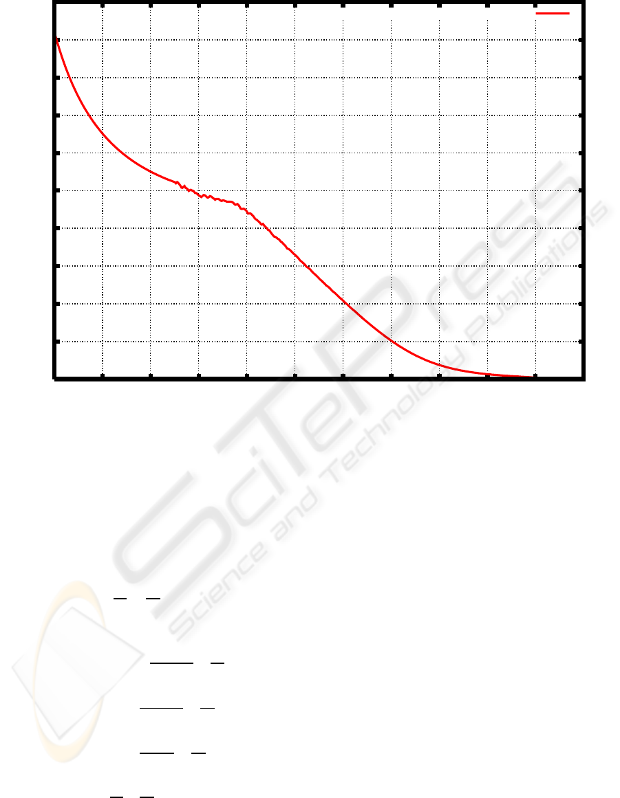
with techniques developed in previous studies. Fig-

ure 3 shows the graph of the function λ(M) based on

the weight distribution before and after cultivation for

three days (Watanabe and Kawai, 2004).

3 TIME FACTOR OF

DEGRADATION RATE

A microbial population grows exponentially in a de-

veloping stage. Since the increase of biodegradability

results from increase of microbial population, it is ap-

propriate to assume that the time factor of the degra-

dation rate σ(t) is an exponential function of time:

σ(t) = e

at+b

. (11)

Then in view of the equation (5)

τ =

σ(s) ds =

as+b

ds =



− 1



Suppose that the weight distribution is given at t =

and t = T

, where 0 < T

< T

, and let

σ(s) ds, (12)

σ(s) ds (13)

It follows that

σ(t) = e

− 1

(14)

and

τ = T

− 1

(15)

Now the equation (13) leads to

= T

− 1

which is equivalent to the equation

h(a) = 0, (16)

where

h(a) =

− 1

−

Since

′

(a) =



− 1



− T



− 1



− 1)

′

(a) > 0 if and only if

− 1

For x > 0

q(x) =

− 1

1− e

−ax

Then

′

(x) =

1− e

−ax

− axe

−ax

(1− e

−ax

)

−ax

− 1− ax)

(1− e

−ax

)

> 0.

BIOSIGNALS 2009 - International Conference on Bio-inspired Systems and Signal Processing

100

120

140

160

180

200

3.1 3.2 3.3 3.4 3.5 3.6 3.7 3.8 3.9 4 4.1 4.2

DEGRADATION RATE [1/DAY]

LOG M

PEG EXOGENOUS DEGRADATION RATE

Figure 3: Degradation rate based on the weight distribution of PEG before and after cultivation of a microbial consortium E1

for three days.

It follows that the q(x) is a strictly increasing

function, and it follows that h

′

(a) > 0.

It is easily seen that

lim

a→∞

h(a) = ∞

Suppose that

(17)

Then by L’Hospital’s rule

lim

a→0+

h(a) = lim

a→0+



− 1

−



= lim

a→0+

− 1

−

= lim

a→0+

−

< 0

(18)

It follows that the condition (17) is a necessary and

sufﬁcient condition for the equation (16) to have a

unique positive solution.

In order to determine a and b, the values of T

, T

, and T

must be set. Let T

= T

= 3. The

initial value problem (6), (7) was solved numerically

with the degradation whose graph is shown in Figure

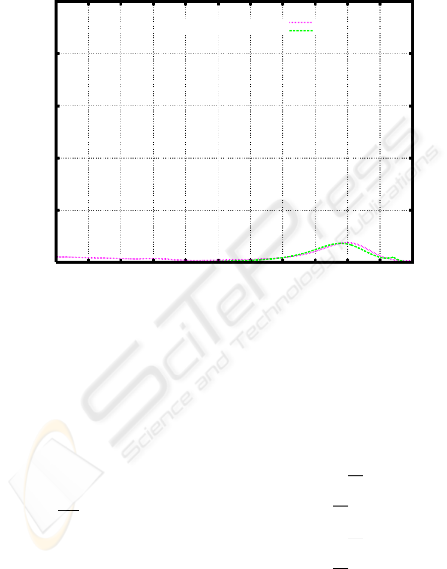
3 to ﬁnd the weight distribution at τ = 30 (Figure 4).

Figure 4 also shows the weight distribution after cul-

tivation for ﬁve days.

Figure 4 shows that it is appropriate to set T

= 5

and T

= 30. Figure 5 shows the graph of h(a) with

those values of parameters.

Figure 5 shows that there is a unique solution of

the equation (16). It was solved numerically with the

Newton’s method, and a numerical solution, which

was approximately equal to 1.136176 was found.

MODELING AND SIMULATION OF BIODEGRADATION OF XENOBIOTIC POLYMERS BASED ON

EXPERIMENTAL RESULTS

0.005

0.01

0.015

0.02

0.025

3.1 3.2 3.3 3.4 3.5 3.6 3.7 3.8 3.9 4 4.1 4.2

COMPOSITION (%)

LOG M

AFTER 5-DAY CULTIVATION

SIMULATION: 30 DAY

Figure 4: Weight distribution of PEG after cultivation for 30 days according to the time independent model based on the initial

value problem (6), (7), and the degradation rate shown in Figure 3. The experimental result obtained after cultivation for 5

days is also shown.

4 SIMULATION WITH TIME

DEPENDENT DEGRADATION

RATE

Once the degradation rate σ(t)λ(M) are given, the

initial value problem (2) and (3) can be solved di-

rectly to see how the numerical results and the ex-

perimental results agree. Here the initial value prob-

lem was solved numerically with techniques base on

previous results (Watanabe et al., 2003; Kawai et al.,

2004; Watanabe et al., 2004).

Choose a positive integer N and set

∆M =

b− a

= a + i∆M, i = 0, 1,2,· · · ,N.

An approximate solution of the differen-

tial equation (1) at M = M

is denoted by

= w

(t) (i = 0,1,2,· · · ,N). There is a non-

negative integer K and a constant R such that

L = K∆M + R, 0 ≤ R < ∆M, and that the inequalities

i+K

≤ M

+ L < M

i+K+1

hold. Then approximate values of w(t, M

+ L) and

β(M

+ L) can be obtained by using the approxima-

tions

w(t,M

+ L) ≈



1−

∆M



w(t,M

i+K

)

∆M

w(t,M

i+K+1

λ(M

+ L) ≈



1−

∆M



λ(M

i+K

)

∆M

λ(M

i+K+1

Substituting these expressions in the differential

equation (2) and setting M = M

, we obtain the linear

BIOSIGNALS 2009 - International Conference on Bio-inspired Systems and Signal Processing

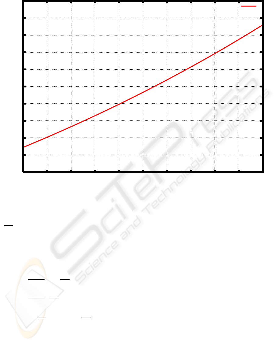
-3

-2.5

-2

-1.5

-1

-0.5

0.5

1.5

1 1.02 1.04 1.06 1.08 1.1 1.12 1.14 1.16 1.18 1.2

h(a)

Graph of h(a)

Figure 5: Graph of h(a) with T

= T

= 3, T

= 5 and T

= 30.

system:

= σ(t) (−α

+ β

i+K

+ γ

i+K+1

i = 0, 1,2,· · · , N.

(19)

The coefﬁcients α

, β

, and γ

are given by

= λ(M

= φ

+ L



1−

∆M



= φ

+ L

∆M



1−

∆M



λ(M

i+K

) +

∆M

λ(M

i+K+1

Approximate values of the degradation rates

λ(M

) can be obtained from the numerical solution

of the inverse problem by the linear approximation.

For all sufﬁciently large M, the oxidation rate be-

comes 0. In particular, we may assume that the last

two terms on the right-hand side of the equation (19)

are absent when i+ K exceeds N, so that the system

(19) becomes a closed system to be solved for un-

known functions w

= w

(t), i = 0,1,2,. .. ,N. In view

of the condition (3), these functions are subject to the

initial condition

(0) = f

= f (M

). (20)

Given the initial weight distribution shown in Fig-

ure 2, the degradation rate λ(M) shown in Figure

3, and the function σ(t) given by the equation (14)

with the value of a obtained numerically, the ini-

tial value problem (19) and (20) was solved numeri-

cally implementingthe forth-orderAdams-Bashforth-

Moulton predictor-corrector in PECE mode in con-

junction with the Runge-Kutta method to generate

approximate solutions in the ﬁrst three steps (Lam-

bert, 1973) by using N = 10000, and a time interval

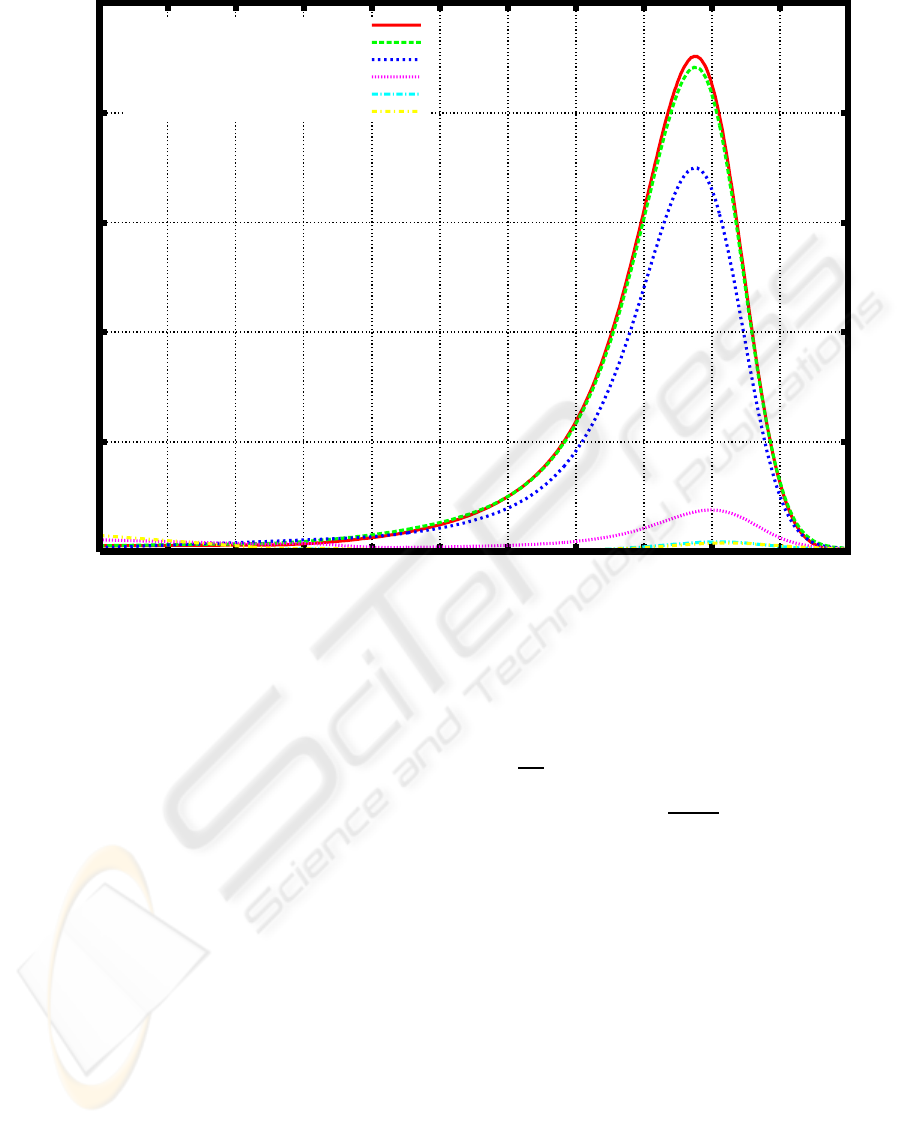
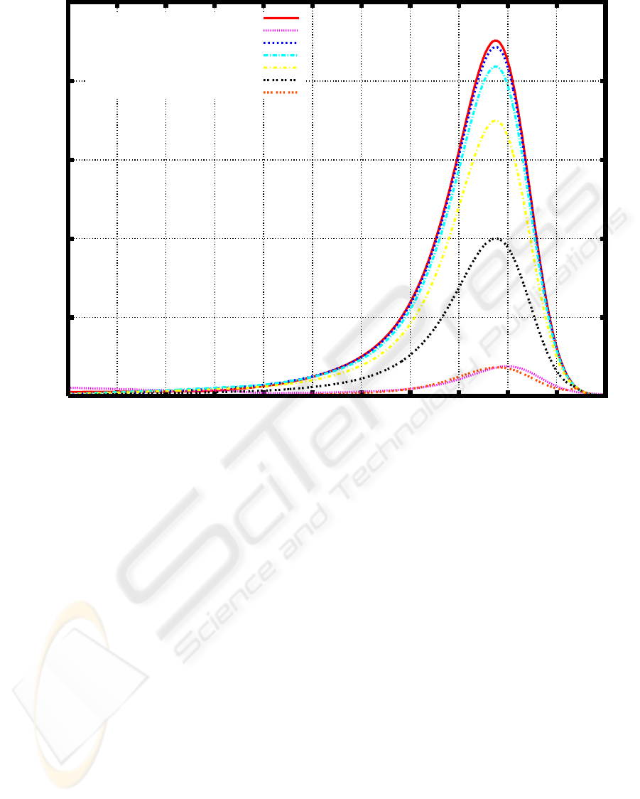
∆t = 5/24000. Figure 6 shows the transition of the

weight distribution during cultivation of the microbial

consortium E-1 for ﬁve days.

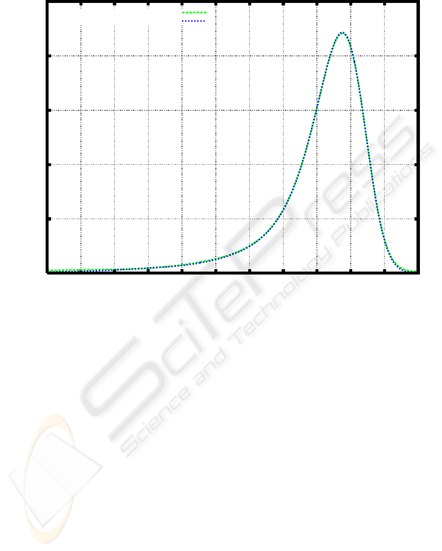
Figure 7 shows the numerical result and the ex-

perimental results for the weight distribution after one

day cultivation of the microbial consortium E1.

MODELING AND SIMULATION OF BIODEGRADATION OF XENOBIOTIC POLYMERS BASED ON

EXPERIMENTAL RESULTS

0.005

0.01

0.015

0.02

0.025

3.1 3.2 3.3 3.4 3.5 3.6 3.7 3.8 3.9 4 4.1 4.2

COMPOSITION (%)

LOG M

BEFORE CULTIVATION

AFTER 5-DAY CULTIVATION

SIMULATION: 1 DAY

SIMULATION: 2 DAY

SIMULATION: 3 DAY

SIMULATION: 4 DAY

SIMULATION: 5 DAY

Figure 6: The weight distribution of PEG before and after 5-day cultivation, and the transition of the weight distribution based

on the initial value problem (2), (3) with σ(t) = e

at+b

, a ≈ 1.136176, b = ln





− 1



, T

= T

= 3.

5 DISCUSSION

Early studies of biodegradation of xenobiotic poly-

mers are found in the second half of the 20th cen-

tury. It was found that the linear parafﬁn molecules

of molecular weight up to 500 were utilized by sev-

eral microorganisms (Potts et al., 1972). Oxida-

tion of n-alkanes up to tetratetracontane (C

mass of 618) In 20 days was reported (Haines et al.,

1974). Biodegradation of polyethylene was shown by

measurement of

generation (Albertsson et al.,

1987). The weight distribution of polyethylene be-

fore and after cultivation of the fungus Aspergillus

sp. AK-3 for 3 weeks was introduced into analysis

based on the time dependent exogenous depolymer-

ization model. The transition of weight distribution

for 5 weeks was simulated with the degradation rate

based on the initial weight distribution and the weight

distribution after 3 weeks of cultivation. The numer-

ical result was found to be acceptable in comparison

with an experimental result (Watanabe et al., 2004).

The result shows that the microbial population was

fully developed in 3 weeks, and that the biodegrada-

tion was with the constant rate.

The degradation rate changed over the cultivation

period in the depolymerizationprocesses of PEG. The

development of microbial population accounts for the

increase of degradability overthe ﬁrst ﬁve days of cul-

tivation. In a depolymerization process where the mi-

crobial population becomes an essential factor, it is

necessary to consider the dependence of the degrada-

tion rate on time. The numerical results based on the

time dependent exogenous depolymerization model

show reasonable agreement with the experimental re-

sults. Those results show that it is appropriate to as-

sume that the degradation rate is a product of a time

factor and a molecular factor. It has also been shown

that the molecular factor can be determined by the

weight distribution before and after cultivation exper-

imentally. In the environment or sewer disposal, the

time factor should also depends on other factors such

as temperature or dissolved oxygen. Once those es-

sentials are incorporated into the time dependent fac-

tor, the time dependent exogenous depolymerization

BIOSIGNALS 2009 - International Conference on Bio-inspired Systems and Signal Processing

0.005

0.01

0.015

0.02

0.025

3.1 3.2 3.3 3.4 3.5 3.6 3.7 3.8 3.9 4 4.1 4.2

COMPOSITION (%)

LOG M

AFTER 1-DAY CULTIVATION

SIMULATION: 1 DAY

Figure 7: The weight distribution of PEG after 1-day cultivation, and the weight distribution based on the initial value problem

(2), (3) with σ(t) = e

at+b

, a ≈ 1.136176, b = ln





− 1



, T

= T

= 3, t = 1.

model and the techniques based on the model should

be applicable to assess biodegradability of xenobiotic

polymers.

REFERENCES

Potts, J.E., Clendinning, R.A., Ackart W.B. and Niegishi,

W.D., The biodegradability of synthetic polymers,

Polym Preprints 1972; 13; 629-34.

Haines, J.R. and Alexander, M., Microbial degradation of

high-molecular-weight alkanes, Appl Microbiol 1974;

28; 1084-5.

Albertsson, A-C, Andersson SO and Karlsson, S, The

mechanism of bioidegradation of plyethylene, Polym

Degrd Stab 1987; 18; 73-87.

Fusako Kawai, Masaji Watanabe, Masaru Shibata, Shi-

geo Yokoyama, Yasuhiro Sudate, Experimental anal-

ysis and numerical simulation for biodegradability of

polyethylene, Polymer Degradation and Stability 76

(2002) 129-135.

Masaji Watanabe, Fusako Kawai, Masaru Shibata, Shigeo

Yokoyama, Yasuhiro Sudate, Computational method

for analysis of polyethylene biodegradation, Journal

of Computational and Applied Mathematics, Volume

161, Issue 1, 1 December 2003, 133-144.

Fusako Kawai, Biodegradability and chemical structure of

polyethers, Kobunshi Ronbunshu, 50(10), 775-780

(1993) (in Japanese).

Fusako Kawai, Breakdown of plastics and polymers by

microorganisms, Advances in Biochemical Engineer-

ing/Biotechnology, Vol. 52, 151-194 (1995).

F. Kawai, Microbial degradation of polyethers, Applied Mi-

crobiology and Biotechnology (2002) 58:30-38.

Lambert, J. D., Computational Methods in Ordinary Differ-

ential Equations, John Wiley Sons, Chichester, 1973.

Fusako Kawai, Masaji Watanabe, Masaru Shibata, Shigeo

Yokoyama, Yasuhiro Sudate, Shizue Hayashi, Com-

parative study on biodegradability of polyethylene

wax by bacteria and fungi, Polymer Degradation and

Stability 86 (2004), 105-114.

Masaji Watanabe, Fusako Kawai, Masaru Shibata, Shigeo

Yokoyama, Yasuhiro Sudate, Shizue Hayashi, Analyt-

ical and computational techniques for exogenous de-

polymerization of xenobiotic polymers, Mathematical

Biosciences 192 (2004) 19-37.

F. Kawai, Xenobiotic polymers, in: T. Imanaka, ed., Great

Development of Microorganisms, (NTS. Inc., Tokyo,

2002) 865-870 (in Japanese).

MODELING AND SIMULATION OF BIODEGRADATION OF XENOBIOTIC POLYMERS BASED ON

EXPERIMENTAL RESULTS

M. Watanabe, F. Kawai, Numerical simulation of microbial

depolymerization process of exogenous type, Proc.

of 12th Computational Techniques and Applications

Conference, CTAC-2004, Melbourne, Australia in

September 2004, Editors: Rob May and A. J. Roberts,

ANZIAM J. 46(E) pp.C1188–C1204, 2005. (http://

anziamj.austms.org.au/V46/CTAC2004/Wata)

M. Watanabe, F. Kawai, Mathematical study of the

biodegradation of xenobiotic polymers with ex-

perimental data introduced into analysis, Proceed-

ings of the 7th Biennial Engineering Mathemat-

ics and Applications Conference, EMAC-2005,

Melbourne, Editors: Andrew Stacey and Bill

Blyth and John Shepherd and A. J. Roberts,

ANZIAM J. 47 pp.C665–C681, 2007. (http:// anzi-

amj.austms.org.au/V47EMAC2005/Watanabe)

Masaji Watanabe, Fusako Kawai, Numerical study of

biodegradation of xenobiotic polymers based on ex-

ogenous depolymerization model with time dependent

degradation rate, Journal of the Faculty of Environ-

mental Science and Technology, Okayama University,

Vol. 12, No. 1, pp. 1-6, March 2007.

BIOSIGNALS 2009 - International Conference on Bio-inspired Systems and Signal Processing