A COMPUTATIONAL SALIENCY MODEL INTEGRATING

SACCADE PROGRAMMING

Tien Ho-Phuoc, Anne Gu´erin-Dugu´e and Nathalie Guyader

GIPSA-lab/Department of Images and Signals, 961 rue de la Houille Blanche, F - 38402 Saint Martin d’H`eres cedex, France

Keywords:

Saccade programming, Saliency map, Spatially variant retinal resolution.

Abstract:

Saliency models have showed the ability of predicting where human eyes ﬁxate when looking at images.

However, few models are interested in saccade programming strategies. We proposed a biologically-inspired

model to compute image saliency maps. Based on these saliency maps, we compared three different saccade

programming models depending on the number of programmed saccades. The results showed that the strategy

of programming one saccade at a time from the foveated point best matches the experimental data from free

viewing of natural images. Because saccade programming models depend on the foveated point where the

image is viewed at the highest resolution, we took into account the spatially variant retinal resolution. We

showed that the predicted eye ﬁxations were more effective when this retinal resolution was combined with

the saccade programming strategies.

1 INTRODUCTION

Eye movement is a fundamental part of human vi-

sion for scene perception. People do not look at all

objects at the same time in the visual ﬁeld but se-

quentially concentrate on attractive regions. Visual

information is acquired from these regions when the

eyes are stabilized (Egeth and Yantis, 1997; Hender-

son, 2003). Psychophysical experiments with eye-

trackers provide experimental data for both behav-

ioral and computational models to predict the attrac-

tive regions.

Computational models are in general divided into

two groups: task-independent models (bottom-up)

and task-dependent models (top-down). Most mod-

els describe bottom-up inﬂuences to create a saliency

map for gaze prediction. They areinspired by the con-

cept of the Feature Integration Theory of Treisman

and Gelade (Treisman and Gelade, 1980) and by the

ﬁrst model proposed by Koch and Ullman (Koch and

Ullman, 1985). The most popular bottom-up saliency

model was proposed by Itti (Itti et al., 1998).

Eye movement experimental data consists, in gen-

eral, of ﬁxations and saccades. Most models were

usually evaluated with distribution of ﬁxations rather

than distribution of saccade amplitudes (in this paper,

saccade distribution

will be used to refer to distribu-

tion of saccade amplitudes). In order to evaluate more

precisely human saccades, saliency prediction must

be included inside a spatio-temporal process, even if

we consider only a bottom-up visual saliency map

from low-level features based on still images. A ques-

tion can be asked: is visual saliency evaluated again

at each ﬁxation, or not?

Some studies showed that the saccadic system can

simultaneously program two saccades to two different

spatial locations (McPeek et al., 2000). This means

that from one foveated point, the next two saccades

are programmed in parallel; this is called the

con-

current processing

of saccades. Moreover, another

study (McPeek et al., 1998) showed that when sub-

jects are explicitly instructed to make a saccade only

after the current information at the fovea has been

analyzed, they have difﬁculty using this strategy. In

this paper, we consider different saccade program-

ming strategies during free viewing of natural im-

ages and we answer the questions: Do subjects make

one saccade at a time, programming the next sac-

cade from the current foveated point? Or do sub-

jects program the next two saccades from the cur-

rent foveated point? To answer these questions, we

tested two different models depending on the corre-

sponding number of programmed saccades from one

foveated point (cf. section 2.4). These two mod-

els were compared with the baseline model in which

all ﬁxations were predicted from the same foveated

point. The mechanism of saccade programming will

be discussed through our experimental results, as it is

still an open question.

Saccade programming models are greatly linked

Ho-Phuoc T., Guérin-Dugué A. and Guyader N. (2009).

A COMPUTATIONAL SALIENCY MODEL INTEGRATING SACCADE PROGRAMMING.

In Proceedings of the International Conference on Bio-inspired Systems and Signal Processing, pages 57-64

DOI: 10.5220/0001535500570064

 SciTePress

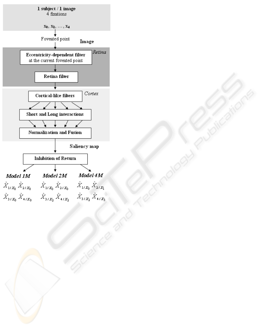
Figure 1: Functional description of the three saccade pro-

gramming models proposed.

to image resolution when it is projected on the retina.

The image on the fovea is viewed at higher resolu-

tion compared to the peripheral regions. This en-

hances the saliency of the region around the foveated

point. The spatial evolution of visual resolution is

one of the consequences of the non-uniform den-

sity of photoreceptors at retina level (Wandell, 1995).

When comparing experimental and predicted scan-

paths, Parkhurst (Parkhurst et al., 2002) noticed an

important bias on saccade distribution. The predicted

saccade distribution is quite uniform, contrary to the

experimental one where ﬁxations are indeed located

on average near the foveated point. The decrease of

visual resolution on the peripheral regions contributes

to an explanation of this effect. In (Parkhurst et al.,

2002), this property was integrated in the model at

the ﬁnal stage (multiplication of the saliency map by

a gaussian function).

In our model, we implement the decreasing den-

sity of photoreceptors as the ﬁrst cause of this in-

homegeneous spatial representation. The output of

photoreceptors encodes spatial resolution depending

on eccentricity, given a parameter of resolution de-

cay (Geisler and Perry, 1998). While this parameter

inﬂuents low level retina processing, we intend to go

further in varying its value to mesure its impact on

high level visual processing, i.e. including the ﬁrst

steps of the visual cortex. Similarly, in (Itti, 2006),

they noticed that the implementation of the spatially

variant retinal resolution improved the ability of ﬁx-

ation prediction for dynamic stimuli (video games),

but the question of saccade programming was not ad-

dressed. Here, we show that this positive effect of

ﬁxation prediction is even signiﬁcant with static vi-

sual stimuli in combination with saccade program-

ming models.

Consequently, the proposed models are dynamic

ones as the high resolution regions, corresponding to

the fovea, change temporally according to the scan-

path. Three saccade programming strategies are ana-

lyzed. Experimental results show the interest of this

approachwith spatially variant retinal resolution. The

models are described in section 2. Section 3 presents

the experiment of free viewing to record eye ﬁxations

and saccades, and the evaluationof the proposed mod-

els. Discussion is drawn in section 4.

2 DESCRIPTION OF THE

PROPOSED MODELS

Our biologically-inspired models (Fig. 1) consist of

one or more saliency maps in combination with sac-

cade programming strategies. The model integrates

the bottom-up pathway from low-level image prop-

erties through the retina and primary visual cortex to

predict salient areas. The retina ﬁlter plays an impor-

tant role: implementing non-linear response of pho-

toreceptors and then, spatially variant resolution. The

retinal image is then projected into a bank of cortical-

like ﬁlters (Gabor ﬁlters) which compete and interact,

to ﬁnally produce a saliency map. This map is then

used with a mechanism of “Inhibition of Return” to

create the saccade programming model. All these el-

ements are described below.

2.1 Retina Filter

In (Beaudot et al., 1993) the retina is modeled quite

completely according to its biological functions: spa-

tially variant retinal resolution, luminance adaptation

and contrastenhancement. These three characteristics

are taken into account while usually a simple modelis

BIOSIGNALS 2009 - International Conference on Bio-inspired Systems and Signal Processing

used such as a function of difference of Gaussians (Itti

et al., 1998).

Spatially variant retinal resolution

: Since the den-

sity of photoreceptors decreases as eccentricity from

the fovea increases(Wandell, 1995), the bluringeffect

increases from the fovea to the periphery and is re-

ﬂected by an eccentricity-dependentﬁlter. The cut-off

frequency f

of this ﬁlter decreases with eccentricity

ecc expressed in degree (Fig. 2a). The variation of the

cut-off frequency (Eq. 1) is adapted from (Geisler and

Perry, 1998; Perry, 2002):

(ecc) = fmax

α+ |ecc|

, (1)

where α is the paramater controlling the resolution

decay, and fmax

the maximal cut-off frequency in

the fovea. Biological studies showed that α is close to

2.3

◦

(Perry, 2002). Figure 2b shows an example of an

image ﬁltered spatially at the center with α = 2.3

◦

Luminance adaptation

: Photoreceptors adapt to a

varying range of luminance and increase luminancein

dark regionswithout saturation of luminance in bright

ones. They carry out a compression function (Eq. 2) :

y = y

max

x+ x

, (2)

where x is the luminance of the initial image, x

rep-

resents its average local luminance, y

max

a normaliza-

tion factor and y the photoreceptor output (Beaudot

et al., 1993).

Contrast enhancement

: The output of horizontal

cells, the low-pass response of photoreceptors, passes

throughbipolar cells and then, throughdifferent types

of ganglion cells: parvocellular, magnocellular and

koniocellular cells. We only consider the two princi-

pal cells: parvocellular and magnocellular. Parvocel-

lular cells are sensitive to high spatial frequency and

can be modeled by the difference between photore-

ceptors and horizontal cells. Therefore, they enhance

the initial image contrast and whiten its energy spec-

trum (Fig. 5b). Magnocellular cells respond to lower

spatial frequency and are modeled by a low-pass ﬁlter

like horizontal cells.

In human visual perception, we know that low fre-

quencies precede high frequencies (Navon, 1977). In

our model, we do not take into account this tempo-

ral aspect. However, as both low and high frequency

components are necessary for a saliency map, we

compute the retina output as a linear combination of

the parvocellularand magnocellular outputs (Fig. 5b).

(a) (b)

Figure 2: (a) Normalized cut-off frequency as function of

eccentricity for different values of α controlling the resolu-

tion decay. (b) An example of the output of the eccentricity-

dependent ﬁlter with α = 2.3

◦

, the foveated point is at the

image center (marked with the cross).

2.2 Cortical-Like Filters

2.2.1 Gabor Filters

Retinal image is transmitted to V1 which processes

signals in different frequencies, orientations, colors

and motion. We only consider the frequency and ori-

entation decomposition carried out by complex cells.

Among several works modeling responses of these

cells, Gabor ﬁlters are evaluated as good candidates.

A set of Gabor ﬁlters is implemented to cover all ori-

entations and spatial frequencies in the frequentialdo-

main. A ﬁlter G

i, j

(Eq. 3) is tuned to its central ra-

dial frequency f

at the orientation θ

. There are N

orientations and N

radial frequencies (N

= 8 and

= 4). The radial frequency is such as f

= 0.25

and f

j− 1

, j = N

,..,2. The standard deviations

of G

i, j

are σ

i, j

and σ

i, j

in the radial direction and its

perpendicular one, respectively. σ

i, j

is chosen in such

a way that ﬁlters G

i, j

and G

i, j− 1

are tangent at level

of 0.5. We notice that the choice of the standard de-

viations inﬂuences the predicted saliency map. We

choose σ

i, j

= σ

i, j

, which is justiﬁed in the next sec-

tion.

i, j

(u,v) = exp

(

−

′

− f

)

2(σ

i, j

)

′2

2(σ

i, j

)

(3)

with:



′

= ucos(θ

) + vsin(θ

)

′

= vcos(θ

) − usin(θ

)

where u (respectively v) is the horizontal (respectively

vertical) spatial frequency. Then, for each channel,

complex cells are implemented as the square ampli-

tude of the Gabor ﬁlter output, providing the energy

maps e

i, j

A COMPUTATIONAL SALIENCY MODEL INTEGRATING SACCADE PROGRAMMING

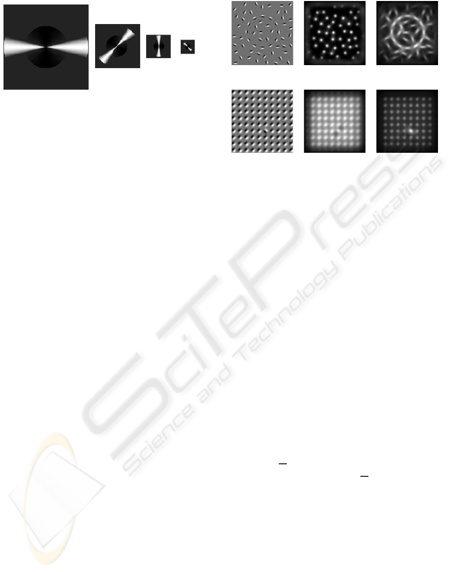
Figure 3: Example of butterﬂy masks with different orien-

tations and scales.

2.2.2 Interaction between Filters

The responses of neurons in the primary visual cor-

tex are inﬂuenced in the manner of excitation or in-

hibition by other neurons. As these interactions be-

tween neurons are quite complex, we only consider

two types of interactions based on the range of recep-

tive ﬁelds (Hansen et al., 2001).

Short interactions are the interactions among neu-

rons having overlapping receptive ﬁelds. They occur

with the same pixel in different energy maps (Eq. 4):

i, j

= 0, 5.e

i, j− 1

+ e

i, j

+ 0,5.e

i, j+1

− 0,5.e

i+1, j

−0,5.e

i−1, j

. (4)

These interactions introduce inhibition between

neurons of neighboring orientations on the same

scale, and excitation between neurons of the same

orientation on neighboring scales. For the standard

deviations of the cortical-like ﬁlters, if σ

i, j

> σ

i, j

the ﬁlters are more orientation-selective. However,

this choice reduces the inhibitive interaction. So, we

choose σ

i, j

= σ

i, j

The second interactions are long interactions

which occur among colinear neurons of non-

overlapping receptive ﬁelds and are often used for

contour facilitation (Hansen et al., 2001). This inter-

action type is directly a convolution product on each

map m

i, j

to produce an intermediate map m

i, j

. The

convolution kernel is a “butterﬂy” mask b

i, j

(Fig. 3).

The orientation of the mask b

i, j

for the map m

i, j

the orientation θ

, and the mask size is inversely pro-

portional to the central radial frequency f

. The “but-

terﬂy” mask b

i, j

has two parts: an excitatory part b

i, j

in the preferential direction θ

and an inhibitive one

−

i, j

in all other directions. It is normalized in such

a way that its summation is set to 1. Figure 4 (ﬁrst

row) shows the interaction effect for contour facilita-

tion (Fig. 4c).

(a) (b) (c)

(d) (e) (f)

Figure 4: Tests showing the inﬂuence of interaction and nor-

malization steps. The initial images are on the left column.

The corresponding saliency maps are on the center and right

column. First row, interaction effect: (a) Initial image; (b)

without interaction; (c) with interaction. Second row, nor-

malization effect: (d) Initial image; (e) without normaliza-

tion; (f) with normalization.

2.3 Normalization and Fusion

Intermediate maps m

i, j

must be normalized before

fusion. Moreover, an object is more salient if it is

different in comparison to its neighbors. We use

the method proposed by L. Itti (Itti et al., 1998) to

strengthen intermediate maps. Then, the maps are

thresholded. Figure 4 (second row) representsthe role

of the normalization step in reinforcing the ﬁlter out-

put where a Gabor patch is different from the back-

ground (Fig. 4f).

The normalization of each map is carried out as

follows:

• Normalize the intermediate map in [0, 1]

• Let us designate m

∗

i, j

the maximal value of map

i, j

and

i, j

its average. Then, the value at each

pixel is multiplied by (m

∗

i, j

−

i, j

)

• Set to zero all the values which are smaller than

20% of the maximal value.

Finally, all intermediate maps are summed up

in different orientations and frequencies to obtain a

saliency map. Examples of retinal image and saliency

map are given in Fig. 5.

2.4 Saccade Programming

Our models predict the ﬁrst four ﬁxations as an ex-

tension of the study in (McPeek et al., 2000) (two

BIOSIGNALS 2009 - International Conference on Bio-inspired Systems and Signal Processing

(a) Initial image (b) Retinal image

Figure 5: Examples of retinal output, saliency map and hu-

man ﬁxations for a part of an image used in the experiment.

saccades or two ﬁxations). The ﬁxations are pre-

dicted (and consequently the saccades) from the out-

put saliency map by implementing a simple mech-

anism of “Inhibition of Return” (IOR). We have

deﬁned three saccade programming models, called

“1M”, “2M” and “4M” (Fig. 1). The “1M” model

has often been used with the hypothesis that all ﬁxa-

tions can be predicted from the same foveated point

at the image center. Here, we tested two other models

where each foveated point allows the next or the next

two ﬁxations to be predicted (“4M” or “2M”, respec-

tively). Let us explain ﬁrst the IOR mechanism with

the “1M” model which is considered as the baseline

model. The ﬁrst ﬁxation is chosen as the pixel which

has the maximal value on the saliency map. Then, this

ﬁxation becomes the foveated point to predict the sec-

ond saccade. Hence, the second ﬁxation is chosen as

the pixel of maximal value after inhibiting the surface

around the foveated point (radius of 1

◦

). This mecha-

nism continues for the third and fourth ﬁxations. For

the “2M” and “4M” models, the IOR mechanism is

applied in the same manner as for the “1M” model

except that the four ﬁxations are predicted from more

than one saliency map (see below).

In the “1M” model, the eccentricity-dependentﬁl-

ter is applied only once to the center X

of images (be-

cause during the eye movement experiment, images

appeared only if subjects were looking at the center of

the screen). Then, a saliency map is computed from

this foveated point to predict four ﬁxations

1/X

2/X

3/X

4/X

by using the IOR mechanism. For

the “2M” model, the eccentricity-dependent ﬁlter is

applied ﬁrst to the center X

, as for the “1M” model,

to predict the ﬁrst two ﬁxations (on the ﬁrst saliency

map)

1/X

2/X

; then, the eccentricity-dependent

ﬁlter is applied again to the second ﬁxation for pre-

dicting the next two ﬁxations (on the second saliency

map)

3/X

4/X

. Because the second ﬁxation is dif-

ferent from one subject to another we take into ac-

count the second ﬁxation X

of each subject for each

image. The “4M” model does the same by applying

the eccentricity-dependent ﬁlter and calculating the

saliency map for each ﬁxation of each subject (four

saliency maps are sequentially evaluated).

3 EXPERIMENTAL EVALUATION

3.1 Eye Movement Experiment

We ran an experiment to obtain the eye scanpaths of

different subjects when they were looking freely at

different images. Figure 5d shows the ﬁxations of all

subjects on a part of an image. The recording of eye

movements served as a method to evaluate our pro-

posed model of visual saliency and saccade program-

ming.

Participants

: Eleven human observers were asked

to look at images without any particular task. All par-

ticipants had normal or corrected to normal vision,

and were not aware of the purpose of the experiment.

Apparatus

: Eye tracking was performed by an

Eyelink II (SR Research). We used a binocular

recording of the pupils tracking at 500Hz. A 9-point

calibration was made before each experiment. The

velocity saccadic threshold is 30

◦

/ s and the acceler-

ation saccadic threshold is 8000

◦

/ s

Stimuli

: We chose 37 gray level images (1024×

768 pixels) with various contents (people, landscapes,

objects or manufactural images).

Procedure

: During the experiment, participants

were seated with their chin supported in front of a

21” color monitor (75 Hz refresh rate) at a viewing

distance of 57 cm (40

◦

× 30

◦

usable ﬁeld of view).

An experiment consisted in the succession of three

items : a ﬁxation cross in the center of the screen,

followed by an image during 1.5 s and a mean grey

level screen for 1 s. It is important to note that the

image appeared only if the subject was looking at the

ﬁxation cross; we ensured the position of the eyes be-

fore the onset of images. Subjects saw the same 37

images in a random order.

We analyzed the ﬁxations and saccades of the

guiding eye for each subject and each image.

A COMPUTATIONAL SALIENCY MODEL INTEGRATING SACCADE PROGRAMMING

3.2 Criterion Choice for Evaluation

The qualities of the model, moreprecisely the saccade

programming strategy and the eccentricity-dependent

ﬁlter, are evaluated with the experimental data (ﬁxa-

tions and saccades). This evaluation allows to test the

predicted salient regions and the saccade distribution.

Firstly, the three models “1M”, “2M” and “4M”

are used to test saccade programming strategies. The

evaluation protocol as in (Torralba et al., 2006) is to

extract from a saliency map the most salient regions

representing 20% of the map surface. Let us call each

ﬁxation “correct ﬁxation” (respectively “incorrect ﬁx-

ation”) if the ﬁxation is inside (respectively outside)

these predicted salient regions. The ratio R

(i,s) of

“correct ﬁxation” for an image i and a subject s is

given below:

(i,s) =

inside

all

.100, (5)

where N

inside

is the number of ﬁxations inside the

salient regions and N

all

is the total number of ﬁxa-

tions.

The average ratio of correct ﬁxations of all cou-

ples (subject × image) is computed. Particularly for

each couple, in the “1M” model, one saliency map

is used to calculate correct ﬁxation index for the ﬁrst

four ﬁxations. In the “2M” model, the ﬁrst saliency

map is used for the ﬁrst two ﬁxations and the second

map for the next two ﬁxations (Fig. 1). Similarly for

the “4M” model, each saliency map is used for the

corresponding ﬁxation. It is noticed that in the “1M”

model, the saliency map of each image is identical for

all subjects (whose foveated point is always at the im-

age center). However, it is no longer the case for the

“2M” or “4M” model where a saliency map depends

on the foveated points of a subject.

Secondly, from the most suitable saccade pro-

gramming strategy chosen above, the predicted sac-

cade distribution for the ﬁrst four saccades is com-

puted and compared with the emperical one from our

experimental data. It has been shown that the parame-

ter α (Eq. 1) which ﬁts the experimental data based on

contrast threshold detection when presenting eccen-

tred gratings is around 2.3

◦

(Perry, 2002). Here, by

varying the α values, the expected effects are: (i) this

parameter must have a great inﬂuence on saccade dis-

tribution and (ii) the best value would be in the same

order of magnitude as 2.3

◦

3.3 Results

3.3.1 Evaluation of the Three Saccade

Programming Models

For saccade programming, Fig. 6 shows the criterion

of correct ﬁxations R

as a function of ﬁxation order

with ﬁve α values (0.5

◦

, 1

◦

, 2

◦

, 4

◦

and inﬁnity) for

the three models. R

of the ﬁrst ﬁxation is identical

for these three models because of the same starting

foveated point. It is also the case for R

of the sec-

ond ﬁxation in “1M” and “2M”, and R

of the third

ﬁxation in “2M” and “4M”. R

for all three models

has the same global trend: decrease with ﬁxation or-

der. The R

ratio is greater for the “4M” model in

comparison to the “1M” model for all ﬁxations. It re-

sults from the reinitialization of the foveated point. In

the “2M” model, an intermediate of the two previous

ones, the increase of R

from the second to third ﬁx-

ation is also explained by this reinitialization. More-

over, the decrease at the second and fourth ﬁxation (in

“2M”) presents necessity of the reinitialization, but at

each ﬁxation. The slower decrease of R

in “4M” is

also coherent with this interpretation.

The α parameter also inﬂuences the quality of the

predicted regions. Saliency models including spa-

tially variant retinal resolution give better results than

the model with constant resolution for the ﬁrst four

ﬁxations (t-test, p < 0.005, except the cases α = 0.5

◦

and α = 1

◦

for the third ﬁxation). However, among

α = 0.5

◦

, α = 1

◦

, α = 2

◦

and α = 4

◦

there is no sig-

niﬁcant difference except for the ﬁrst ﬁxation. At

this ﬁxation, there is no difference between R

cases 0.5

◦

and 1

◦

but they are signiﬁcantly greater

than those in cases 2

◦

and 4

◦

(F(3,1612) = 10.45,

p < 0.005).

3.3.2 Conﬁguration of the

Eccentricity-Dependent Filter

To evaluate the inﬂuence of the spatially variant reti-

nal resolution on the saccade distribution, the same

ﬁve α values are tested with the “4M” model which

ﬁts best the human ﬁxations. We observe a great in-

ﬂuence of α on saccade distribution. Figure7 presents

the experimental saccade distribution and those of the

“4M” model according to the ﬁve α values. The

distribution is very narrow with α = 0.5

◦

(Fig. 7b),

larger with greater α, and tends to a uniform dis-

tribution when α tends to inﬁnity (Fig. 7f). The

effect of the spatially variant retinal resolution can

be shown through these distributions, concerning not

only the dispersion but also the position of the max-

imum mode. Let us consider only two characteris-

tics of the saccade distribution : form and position

BIOSIGNALS 2009 - International Conference on Bio-inspired Systems and Signal Processing

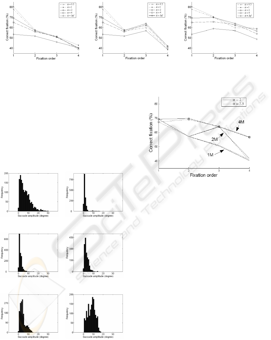
(a) “1M” (b) “2M” (c) “4M”

Figure 6: R

as a function of ﬁxation order of the three models with different α values.

of the maximum mode. By varying α, we can adapt

either distribution form or mode position. However,

it is difﬁcult to ﬁt at the same time both form and

mode position just only by adjusting one parameter

(α here). Hence, the best parameter α is chosen as

the best qualitative compromise between the distribu-

tion form and mode position. Among these α val-

ues, according to the mode position, the distribution

with α = 2

◦

has the same mode position of about 2.1

◦

as the experimental distribution. This distribution de-

creases progressively while eccentricity increases.

(a) Human (b) “4M” with α = 0.5

◦

(d) “4M” with α = 2

◦

(e) “4M” with α = 4

◦

(f) “4M” with α = Inf

Figure 7: Saccade distribution of the experimental data and

the “4M” model according to different values of α.

Figure 8: Comparison of R

between α = 2

◦

and α = 2.3

◦

for the three models.

Indeed, when varying the α parameter, we notice

a continuous effect both on the ratio R

of “correct

ﬁxation” and saccade distribution. The results from

the simulations with α = 2.3

◦

are very close to those

obtained with α = 2

◦

(Fig. 8). By lack of space, the

saccade distribution of the “4M” model for α = 2.3

◦

which is almost the same as for α = 2

◦

, is not shown.

4 DISCUSSION

Firstly, all three models have the ratio of correct ﬁx-

ation decreasing according to the ﬁxation order. This

fact can be explained by the inﬂuence of top-down

mechanisms which arise late and reduce the role of

bottom-up in visual attention. In reality, as time

passes, ﬁxations of different subjects are more dis-

persive and subject-dependent. However, the inﬂu-

ence of bottom-up still persists and the percentage of

correct ﬁxations is much higher than by chance in all

three models. This conﬁrms the role of bottom-up in

visual attention even with the increasing presence of

top-down.

The result of this study seems not to support pro-

A COMPUTATIONAL SALIENCY MODEL INTEGRATING SACCADE PROGRAMMING

gramming of several saccades in parallel. In fact,

we tested three models: the “1M” model program-

ming four saccades in parallel from the same foveated

point, the “2M” model programming two saccades in

parallel and the “4M” model programming only one

saccade at a time. This study showed that the “1M”

model is not realistic and the “4M” model seems to be

the most realistic. The behaviour of the “2M” model

illustrates that recomputing saliency in updating the

foveated point is beneﬁcial. The best performance

comes however from the “4M” model presenting ef-

fectiveness of the reinitialization at each ﬁxation. We

can conclude that saccade programming in parallel

seems not to be used by subjects when they have to

look freely at natural images.

Secondly, this study shows the positive effect of

the spatially variant retinal resolution on the pre-

diction quality. Whatever the saccade programming

strategy is, the models including the spatially vari-

ant retinal resolution greatly outperform the models

with constant resolution in terms of the quality of

ﬁxation prediction and saccade distribution. The pa-

rameter α which controls the resolution decrease has

an important impact on saccade distribution (disper-

sion and mode position). Moreover, we found the

expected range of value for this parameter using our

model to compute saliency maps. We also notice that

if we have the same mode position, the dispersion of

the saccade distribution remains smaller on predicted

data than on experimental data, as we only consider a

bottom-up model and we have only one parameter to

adjust.

In our models, a foveated point for the next sac-

cade is selected from subjects’ ﬁxations instead of be-

ing looked for in the present saliency map. While ﬁx-

ations are different from one subject to another, the

model is a subject-dependent model. If we want to go

further in creating a more general model of predict-

ing eye movements automatically, the model would

take into account human task, for example catego-

rization or information search, and hence passes from

a region-predicting model to a scanpath-predicting

model.

ACKNOWLEDGEMENTS

This work is partially supported by grants from the

Rhˆone-Alpes Region with the LIMA project. T. Ho-

Phuoc’s PhD is funded by the French MESR.

REFERENCES

Beaudot, W., Palagi, P., and Herault, J. (1993). Realistic

simulation tool for early visual processing including

space, time and colour data. In International Work-

shop on Artiﬁcial Neural Networks, LNCS, volume

686, pages 370–375, Barcelona. Springer-Verlag.

Egeth, H. E. and Yantis, S. (1997). Visual attention: Con-

trol, representation, and time course. In Annual Re-

view of Psychology, volume 48, pages 269–297.

Geisler, W. S. and Perry, J. S. (1998). A real-time foveated

multiresolution system for low-bandwidth video com-

munication. In Human Vision and Electronic Imaging,

Proceedings of SPIE, volume 3299, pages 294–305.

Hansen, T., Sepp, W., and Neumann, H. (2001). Recurrent

long-range interactions in early vision. In S. Wermter,

J. A. and Willshaw, D., editors, Emergent Neural

Computational Architectures Based on Neuroscience,

LNCS/LNAI, volume 2036, pages 139–153.

Henderson, J. M. (2003). Human gaze control in real-world

scene perception. In Trends in Cognitive Sciences,

volume 7, pages 498–504.

Itti, L. (2006). Quantitative modeling of perceptual salience

at human eye position. In Visual Cognition, vol-

ume 14, pages 959–984.

Itti, L., Koch, C., and Niebur, E. (1998). A model of

saliency-based visual attention for rapid scene anal-

ysis. In IEEE Transactions on Pattern Analysis and

Machine Intelligence, volume 20, pages 1254–1259.

Koch, C. and Ullman, S. (1985). Shifts in selective visual

attention: towards the underlying neural circuitry. In

Human Neurobiology, volume 4, pages 219–227.

McPeek, R. M., Skavenski, A. A., and Nakayama, K.

(1998). Adjustment of ﬁxation duration in visual

search. In Vision Research, volume 38, pages 1295–

1302.

McPeek, R. M., Skavenski, A. A., and Nakayama, K.

(2000). Concurrent processing of saccades in visual

search. In Vision Research, volume 40, pages 2499–

2516.

Navon, D. (1977). Forest before trees: the precedence of

global features in visual perception. In Cognitive Psy-

chology, volume 9, pages 353–383.

Parkhurst, D., Law, K., and Niebur, E. (2002). Modeling

the role of salience in the allocation of overt visual

attention. In Vision Research, volume 42, pages 107–

123.

Perry, J. S.(2002). http://ﬁ.cvis.psy.utexas.edu/software.shtml.

Torralba, A., Oliva, A., Castelhano, M. S., and Henderson,

J. M. (2006). Contextual guidance of eye movements

and attention in real-world scenes: The role of global

features in object search. In Psychological Review,

volume 113, pages 766–786.

Treisman, A. and Gelade, G. (1980). A feature integra-

tion theory of attention. In Cognitive Psychology, vol-

ume 12, pages 97–136.

Wandell, B. A. (1995). Foundations of Vision. Stanford

University.

BIOSIGNALS 2009 - International Conference on Bio-inspired Systems and Signal Processing