BANKRUPTCY PREDICTION BASED ON INDEPENDENT
COMPONENT ANALYSIS
Ning Chen
GECAD, Instituto Superior de Engenharia do Porto, Instituto Politecnico do Porto, Portugal
Armando Vieira
Physics Department, Instituto Superior de Engenharia do Porto, Instituto Politecnico do Porto, Portugal
Keywords:
Bankruptcy prediction, Learning vector quantization, Independent component analysis.
Abstract:
Bankruptcy prediction is of great importance in financial statement analysis to minimize the risk of decision
strategies. It attempts to separate distress companies from healthy ones according to some financial indicators.
Since the real data usually contains irrelevant, redundant and correlated variables, it is necessary to reduce the
dimensionality before performing the prediction. In this paper, a hybrid bankruptcy prediction algorithm is
proposed based on independent component analysis and learning vector quantization. Experiments show the
algorithm is effective for high dimensional bankruptcy data and therefore improve the capability of prediction.
1 INTRODUCTION
Bankruptcy prediction is an important issue for
human decision-making in many financial do-
mains (P. Ravi Kumara, 2007). It can be regarded
as a classification task which attempts to separate
distress companies from healthy ones in terms of
some financial and accounting indicators, such as
profitability, solidity and liquidity. Compared to
traditional statistical methods, e.g., linear discrim-
inant analysis (LDA) and multivariate discriminant
analysis (MDA), artificial neuron networks (ANNs)
achieve desirable performance and therefore receive
more and more attentions to solve bankruptcy pre-
diction tasks. The appealing aspect of ANN is char-
acterized by nonlinear modelisation, computational
simplicity and noise insensitivity. It was reported
that among intelligent techniques ANN is the most
widely used family in supervised or unsupervised
manner (P. Ravi Kumara, 2007), e.g., self-organizing
map (SOM) (E. Merkevicius, 2004), learning vec-
tor quantization (LVQ) (K. Kiviluoto, 1997), multi
layer perceptron (MLP) (Armando Vieira, 2003). The
ability of LVQ for bankruptcy prediction has been
demonstrated (K. Kiviluoto, 1997). LVQ is also used
to correct the output of MLP in a hidden layer learn-
ing vector quantization algorithm in order to improve
the quality of prediction (J.C. Neves, 2006).
Due to the complexity of financial statements, a
few indicators are insufficient for bankruptcy predic-
tion, while a large number of indicators lead to the
curse of dimensionality, i.e., the amount of training
data needed increases exponentially with the number
of variables in order to cover the decision space. The
real data usually contains irrelevant, redundant and
correlated variables, not only decreasing the precision
of classification but also consuming a mass of com-
putational time and space. Feature reduction picks
a subset of relevant features to target (selection) or
generates new features from the basic ones (construc-
tion) in order to achieve a more concise and accurate
model (M. Dash, 1997) . It is particularly important
when the number of training data is limited. In the
literature, a number of feature selection methods are
available. In (Tsai, 2008), five well-known statistical
methods, i.e., t-test, correlation matrix, factor anal-
ysis, principle component analysis and stepwise re-
gression are compared based on a MLP classifier for
bankruptcy prediction. Independent component anal-
ysis (ICA) (A. Hyvarinen, 2001) originating from sig-
nal processing is one of the promising methods for
dimensionality reduction and has been used with suc-
cess in many applications (E. Oja, 2000; Bingham,
2001), e.g., financial time series analysis, text mining,
150
Chen N. and Vieira A. (2009).
BANKRUPTCY PREDICTION BASED ON INDEPENDENT COMPONENT ANALYSIS.
In Proceedings of the International Conference on Agents and Artificial Intelligence, pages 150-155
DOI: 10.5220/0001536301500155
Copyright
c
 SciTePress

Figure 1: Algorithm description.
astronomical telescope image processing and wireless
communication.
In this paper, a batch learning vector quantiza-
tion algorithm is used as a classification approach for
bankruptcy prediction according to a number of fi-
nancial indicators. The LVQ algorithm starts from a
trained SOM and learns in batch manner. In data pre-
processing phase, the independent component analy-
sis is applied as a feature construction tool to trans-
form data in high dimensional input space to low di-
mensional ICA space composed of independent com-
ponents. The proposed approach is tested on a French
financial database by cross validation principle. Ex-
perimental results on both balanced and unbalanced
data show that the hybrid algorithm is superior or
comparable to plain LVQ and some well-known clas-
sification algorithms.
The paper is organized as follows. In the next
section, the methodology of LVQ and ICA for
bankruptcy prediction is illustrated. Then the exper-
iments and results are presented. Lastly, the conclu-
sions and future issues are given.
2 METHODOLOGY
The proposed algorithm is motivated by the capability
of LVQ as a classification tool and the ability of ICA
as a dimensionality reduction tool. The algorithm is
processed in two phases as described in Figure 1. In
the first phase, the input vector in original data space
is fed into an ICA preprocessing module given the
number of dimensions remained. The transformed
data in ICA space has less dimensions than original
data while preserving the intrinsic distribution. In the
second phase, the data is input in batch to the LVQ
map for classifier training in a supervised manner.
2.1 ICA
Independent component analysis is a signal process-
ing method to separate a multivariate signal into
independent components under the assumption that
the components are statically independent in non-
Gaussian distribution. Formally, an observed paral-
lel signal x
i
(i = 1,...,n) is a linear mixture of inde-
pendent source signals or factors s
j
( j = 1,...,m) with
mixing coefficients a
i, j
:
x
i
=
m
∑
j=1
a
i, j
s
j
In vector format,
x = As
where x = [x
1
,...,x
n
]
′
, A = (a
i, j
), and s = [s
1
,..,s
m
]
′
.
The basic idea of ICA is to estimate unknown A
and s given the observations x. Alternatively, the in-
dependent components can be calculated:
s = Wx
where W is the inverse matrix of A. The transformed
data in ICA space is of less dimensions and there-
fore easily predicted. In this paper, a fast ICA algo-
rithm (E. Oja, 2000) is used for efficient ICA estima-
tion in a fixed-point iteration scheme.
2.2 LVQ
LVQ is an artificial neural network for supervised
learning usage. It consists of two layers of neurons:
the neurons in input layer receive data from variables
and the neurons in output layer arranged in a regu-
lar grid of one or two dimensions are associated with
input neurons by weight vectors (reference vectors,
or prototypes). The prototypes define the represen-
tative vector of corresponding class regions. During
the training, the prototypes are updated according to
the projection between input data and neurons in or-
der to adjust the class boundary. To get a reasonable
initialization, LVQ usually starts from a trained map
of SOM (Kohonen, 1997). In this paper, a batch LVQ
algorithm is applied for data classification.
Firstly, a SOM is initialized with a number of neu-
rons and trained in an unsupervised way. Then the
neurons are assigned by the majority label principle.
In one batch round, an instance x is selected as in-
put once a time and the Euclidean distance is calcu-
lated between x and each neuron m
i
, then the one of
smallest distance is selected as the best matching unit
(BMU). As a result, x is projected to its BMU c.
c = argmin
i
d(x,m
i
)
After all input are processed, the data is divided
into a number of Voronoi sets: V
i
= {x
k
| d(x
k
,m
i
) ≤
d(x
k
,m
j
),1 ≤ k ≤ n,1 ≤ j ≤ m}. Each Voronoi set is
composed of the instances whose BMU is the corre-
sponding neuron. The prototype is then updated sum-
ming up the impact of all elements in Voronoi sets
BANKRUPTCY PREDICTION BASED ON INDEPENDENT COMPONENT ANALYSIS
151

with the consideration of class matching. Let h
ip
be
the indicative function whose value is 1 if m
p
is the
winner neuron of x
i
and with the same class label to
x
i
, and -1 if m
p
is the winner neuron of x
i
and with
different class label to x
i
, and 0 otherwise. The update
rules are described as:
m
p
(t + 1) =
n
∑
i=1
h
ip
x
i
n
∑
i=1
h
ip
where
h
ip
=



1 if m
p
= BMU(x
i
),class(m
p
) = class(x
i
)
−1 if m
p
= BMU(x
i
),class(m
p
) 6= class(x
i
)
0 otherwise
If the denominator is 0 for some m
p
, no updating
is done. This process is repeated for sufficient itera-
tions until the prototypes are regarded as steady. The
learned map is used for future classification in which
the data is compared with the neuron and assigned by
the class of its BMU.
3 EXPERIMENTAL METHOD
The data used in the experiments comes from the Di-
anan database of French companies, containing the
financial statements during 1998 and 2000. Most
companies are of small or middle size with at least
35 employees. In the total 2056 companies, 583
are labeled by ‘distress’ (declare as bankruptcy or
submit a restructuring plan) and 1473 are labeled as
‘healthy’. Utilizing the inconsistency analysis, 17 in-
dicators are remained with strong correlation to the
class, added by three annual variations of important
ratios (J.C. Neves, 2006). Described in Table 1, the
final data consists of 20 financial ratios followed by
the class label. To study the impact of data balance to
performance, the training data is randomly selected
from the original dataset, with different proportions
of healthy companies compared to bankruptcy com-
panies as 50/50 (DS1), 64/38 (DS2) and 72/28 (DS3)
respectively.
In bankruptcy prediction domain, the traditional
accuracy is insufficient for evaluation due to the dif-
ferent cost of misclassification. Therefore, seven
measures are used for classification evaluation. Type I
error (missing alarm) is the percentage of misclassifi-
cation classifying a bankruptcy company as a healthy
one, while type II error (false alarm) is the percent-
age of misclassification classifying a healthy com-
pany as a bankruptcy one. Overall error is the per-
centage of companies classified incorrectly. Besides,
Table 1: Financial indicators of French companies.
variables description
1 number of employee
2 financial equilibrium ratio
3 equity to stable funds
4 financial autonomy
5 current ratio
6 collection period
7 interest to sales
8 debt ratio
9 financial debt to cash earnings
10 working capital in sales days
11 value added per employee
12 value added to assets
13 EBITDA margin
14 margin before extra items and taxes
15 return on equity
16 value added margin
17 percentage of value added for employees
18 annual variation of debt ratio
19 annual variation of percentage
of value added for employee
20 annual variation of margin before
extra items and taxes
21 class: 0 for ‘healthy’, 1 for ‘bankruptcy’
the OC (overall accuracy) is the percentage of com-
panies classified correctly, BC (bankruptcy classifica-
tion) is the percentage of bankruptcy classified cor-
rectly, BPC (bankruptcy prediction classification) is
the percentage of bankruptcy companies in the to-
tal predicted bankruptcies, WE (weighted efficiency)
is the combination of three accuracy measures. The
error and accuracy measures are defined in Table 2,
where n
ij
denotes the number of companies belong-
ing to group i (0 for healthy and 1 for bankruptcy)
in real classes and group j in predicted classes. The
cross validation technique is employed for perfor-
mance evaluation in terms of error measures and ac-
curacy measures.
Table 2: Evaluation measures.
measures definition
Type I error n
10
/(n
10
+ n
11
)
Type II Error n
01
/(n
01
+ n
00
)
Overall Error (n
10
+ n
01
)/(n
10
+ n
11
+ n
01
+ n
00
)
OC (n
00
+ n
11
)/(n
10
+ n
11
+ n
01
+ n
00
)
BC n
11
/(n
10
+ n
11
)
BPC n
11
/(n
01
+ n
11
)
WE
√
OC ∗BC∗BPC
The LVQ algorithm is implemented in Matlab and
performed with FastICA package (Erkki Oja, 2005).
In summary, the experiments are performed in the fol-
lowing steps:
1. Apply ICA to original data given the number of
dimensions remained;
ICAART 2009 - International Conference on Agents and Artificial Intelligence
152

2. Randomly select a number of healthy companies
from the preprocessed data with the percent ratio
and generate the experimental datasets;
3. Divide the data into 10 folds randomly for cross-
validation: 90% is used for model training, and
the other 10% is used for performance validation;
4. Train LVQ on each training data and then classify
the test data according to the resulting map;
5. Calculate the error and accuracy measures for
classification evaluation;
6. Obtain the average value of measures for distinct
results in cross validation.
4 RESULTS AND DISCUSSION
From the curve shown in Figure 2, the eigenvalues
remained increase monotonously with respect to the
number of dimensions and achieve 99.9% at 15 di-
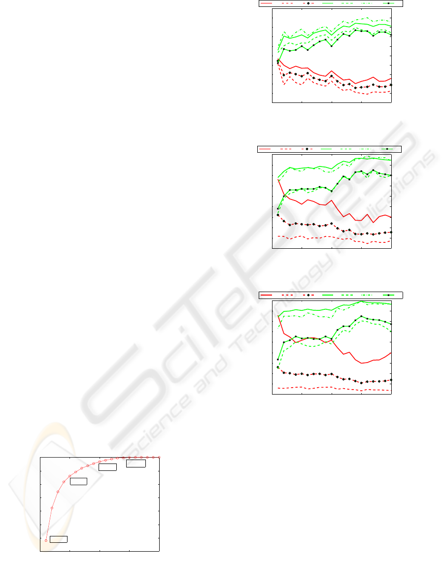
mensions. Figure 3 shows the results at various num-
ber of dimensions remained for classifier construc-
tion on DS1. The default map size of LVQ is de-
termined heuristically by the number of training data
with the side lengths of map grid as the ratio of two
biggest eigenvalues. The error measures decrease dra-
matically at the beginning and amount to the minimal
(e.g., overall error is 0.156 on DS1) nearby 14 dimen-
sions. Increasing further the number of dimensions
does not have any improvement. Meantime, the ac-
curacy measures demonstrate the opposite tendency,
i.e., increase first and amount to maximum at 14 di-
mensions (e.g., WE is 0.77 correspondingly). The
tendency could also be detected from the plot of DS2
(Figure 4) and DS3 (Figure 5). The number of di-
mensions corresponding to the best WE is 14 (DS1),
17 (DS2) and 15 (DS3) respectively. In the following
experiments, we choose the number of dimensions as
the above values.
0 5 10 15 20
30
40
50
60
70
80
90
100
dimension
eigenvalues retained
1:37.96%
5:86.1%
15:99.9%
10:96.8%
Figure 2: Eigenvalues and dimension of ICA.
In Table 3-Table 5, the results of measures for bal-
anced (DS1) and unbalanced (DS2 and DS3) data are
0 5 10 15 20
0
0.1
0.2
0.3
0.4
0.5
0.6
0.7
0.8
0.9
1
dimensions
measures
Err1 Err2 Err OC BC BPC WE
Figure 3: Results of various dimensions on DS1.
0 5 10 15 20
0
0.1
0.2
0.3
0.4
0.5
0.6
0.7
0.8
0.9
dimensions
measures
Err1 Err2 Err OC BC BPC WE
Figure 4: Results of various dimensions on DS2.
0 5 10 15 20
0
0.1
0.2
0.3
0.4
0.5
0.6
0.7
0.8
0.9
dimensions
measures
Err1 Err2 Err OC BC BPC WE
Figure 5: Results of various dimensions on DS3.
given. For all datasets, the proposed Hybrid LVQ
with ICA (approach1) achieves noticeably lower er-
rors (e.g., at least 2% for overall error) and higher ac-
curacy (e.g., at least 4% for weighted efficiency) than
plain LVQ without data preprocessing (approach2).
The former outperforms the latter significantly on
classifying unknown data, indicating ICA is bene-
ficial for dimensionality reduction and consequently
improves the generalization error when the training
data is insufficient. Additionally, utilizing the unbal-
anced data is able to improve type II error, but elim-
inate simultaneously type I error which usually cost
more in real situations. It is also shown that LVQ
with ICA is less biased to unbalanced data than the
plain LVQ.
The map size is one of the most important param-
BANKRUPTCY PREDICTION BASED ON INDEPENDENT COMPONENT ANALYSIS
153

Table 3: Results on DS1.
mea- arrroach1 approach2
sures train test train test
Err1 0.132 0.201 0.172 0.227
Err2 0.059 0.109 0.081 0.142
Err 0.096 0.156 0.126 0.185
OC 0.904 0.844 0.874 0.815
BC 0.868 0.799 0.828 0.773
BPC 0.937 0.879 0.911 0.847
WE 0.86 0.77 0.812 0.73
Table 4: Results on DS2.
mea- arrroach1 arrroach2
sures train test train test
Err1 0.184 0.247 0.22 0.314
Err2 0.038 0.069 0.04 0.066
Err 0.091 0.134 0.105 0.154
OC 0.909 0.866 0.895 0.846
BC 0.816 0.753 0.78 0.686
BPC 0.924 0.860 0.917 0.855
WE 0.83 0.749 0.801 0.704
eters influencing the classifier performance. The re-
sults of different map sizes on DS1 is given in Ta-
ble 6. As the map enlarges from 4 x 3 to 14 x 11, it
performs better on both training and generalization.
When more neurons (27 x 23) are used, the train-
ing error improves slightly while the generalization
error degrades significantly. The results on DS2 and
DS3 are shown in Table 7 and Table 8 respectively.
It can be concluded that the middle size of map grid
is suitable for model construction empirically, while
less units are inadequate for pattern presentation, and
more units leads to overfitting.
Table 9 shows the results obtained on balanced
and unbalanced data sets for Hybrid LVQ and some
well-known classification methods: ZeroR (a baseline
algorithm by simply predicting the majority class in
training data), VFI (voting feature interval classifier),
SMO (sequential minimal optimization algorithm im-
plementing support vector machine), k-nearest neigh-
bors (KNN, the best value of k chosen between 1 and
10), Naive Bayes, and C4.5 decision tree. Among
the seven algorithms, VFI and SMO have poor per-
formance just better than ZeroR in all data sets, fol-
lowed by KNN and Naive Bayes. Superior to the five
algorithms, hybrid LVQ performs well, close to C4.5
in terms of error and accuracy measures. However,
LVQ is a projection method as well as a classification
approach. An appeal of LVQ is the ability to detect
class structure from map visualization which makes it
a useful tool in data mining tasks. Figure 6 presents a
generated map of LVQ, the labels on the left and the
histogram of class distribution on the right. From the
Table 5: Results on DS3.
mea- arrroach1 arrroach2
sures train test train test
Err1 0.209 0.297 0.275 0.417
Err2 0.024 0.033 0.028 0.432
Err 0.076 0.108 0.097 0.152
OC 0.924 0.892 0.903 0.848
BC 0.791 0.703 0.725 0.583
BPC 0.929 0.894 0.909 0.845
WE 0.82 0.748 0.771 0.647
Table 6: Results of different map sizes on DS1.
mea- small:4x3 middle:14x11 big:27x23
sures train test train test train test
Err1 0.3 0.29 0.13 0.2 0.07 0.23
Err2 0.06 0.08 0.06 0.11 0.07 0.18
Err 0.18 0.19 0.1 0.16 0.07 0.2
OC 0.82 0.81 0.9 0.84 0.93 0.78
BC 0.7 0.71 0.87 0.8 0.93 0.77
BPC 0.92 0.91 0.94 0.88 0.93 0.82
WE 0.73 0.73 0.86 0.77 0.9 0.71
Table 7: Results of different map sizes on DS2.
mea- small:8x6 middle:15x13 big:30x26
sures train test train test train test
Err1 0.33 0.37 0.18 0.25 0.1 0.27
Err2 0.03 0.04 0.04 0.07 0.04 0.11
Err 0.14 0.16 0.09 0.13 0.06 0.17
OC 0.87 0.84 0.91 0.87 0.94 0.83
BC 0.67 0.63 0.82 0.75 0.9 0.73
BPC 0.94 0.92 0.92 0.86 0.93 0.78
WE 0.74 0.7 0.83 0.75 0.89 0.69
Table 8: Results of different map sizes on DS3.
mea- small:8x7 middle:16x13 big:31x27
sures train test train test train test
Err1 0.36 0.4 0.21 0.3 0.11 0.31
Err2 0.02 0.03 0.02 0.03 0.02 0.06
Err 0.12 0.14 0.08 0.11 0.05 0.14
OC 0.88 0.86 0.92 0.89 0.95 0.87
BC 0.64 0.6 0.79 0.7 0.89 0.69
BPC 0.92 0.87 0.93 0.89 0.93 0.81
WE 0.72 0.67 0.82 0.75 0.89 0.69
visualization, the healthy companies projected to neu-
rons in the middle of map grid and bankruptcy com-
panies projected to the surrounding neurons.
5 CONCLUSIONS
In this paper, a hybrid LVQ algorithm is presented
to solve the bankruptcy prediction problem. In or-
der to reduce the curse of dimensionality, ICA is used
as a preprocessing tool to eliminate the dimensions
ICAART 2009 - International Conference on Agents and Artificial Intelligence
154

Figure 6: A sample generated LVQ.
Table 9: Results of balanced and unbalanced data sets.
bankruptcy Type I Type II Overall WE
/healthy Error Error Error
50/50
ZeroR 0.604 0.403 0.503 0.312
VFI 0.474 0.03 0.252 0.61
SMO 0.267 0.194 0.231 0.667
KNN 0.271 0.071 0.171 0.742
Naive Bayes 0.304 0.050 0.177 0.731
Hybrid LVQ 0.201 0.109 0.156 0.77
C4.5 0.156 0.130 0.143 0.791
36/64
ZeroR 1 0 0.36 -
VFI 0.667 0.019 0.252 0.476
SMO 0.470 0.047 0.199 0.605
KNN 0.363 0.039 0.156 0.697
Naive Bayes 0.342 0.047 0.153 0.703
Hybrid LVQ 0.247 0.069 0.134 0.749
C4.5 0.172 0.083 0.115 0.789
28/72
ZeroR 1 0 0.28 -
VFI 0.734 0.012 0.214 0.432
SMO 0.566 0.018 0.171 0.571
KNN 0.398 0.028 0.131 0.684
Naive Bayes 0.330 0.047 0.126 0.704
Hybrid LVQ 0.297 0.033 0.108 0.748
C4.5 0.179 0.077 0.104 0.765
in a transformed independent component space. Re-
sults on French companies data demonstrate the pro-
posed algorithm is of higher stability and generaliza-
tion power than plain LVQ without ICA. Regarding
the comparison of seven classification methods, the
hybrid LVQ performs well, only slightly inferior to
C4.5. Since ICA is used as a feature reduction tool in
data preprocessing phase, it could be combined with
other classification tools.
In future work, some strategies, e.g., Neyman-
Pearson criterion are expected to improve the per-
formance of the presented algorithm in cost sensi-
tive situation. The non-uniqueness of different ICA
algorithms will be considered in the evaluation. In
addition, there exist various linear or nonlinear fea-
ture reduction methods, so further investigation is
needed to compare and evaluate their performance for
bankruptcy prediction.
ACKNOWLEDGEMENTS
The authors would like to acknowledge the financial
grant of GECAD/ISEP-Knowledge Based, Cognitive
and Learning Systems (C2007-FCT/442/2006).
REFERENCES
A. Hyvarinen, J. Karhunen, E. O. (2001). Independent com-
ponent analysis. John Wiley & Sons.
Armando Vieira, N. B. (2003). A training algorithm for
classification of high dimensional data. Neurocom-
puting, 50(1):461–472.
Bingham, E. (2001). Topic identification in dynamical text
by extracting minimum complexity time components.
In Proc. 3rd International Conference on Indepen-
dent Component Analysis and Blind Signal Separa-
tion, pages 546–551.
E. Merkevicius, G. Garsva, R. S. (2004). Forecasting of
credit classes with the self-organizing maps. Informa-
tion Technology And Control, Kaunas, Technologija,
4(33):61–66.
E. Oja, K. Kiviluoto, S. M. (2000). Independent compo-
nent analysis for financial time series. In Proc. IEEE
2000 Symp. on Adapt. Systems for Signal Proc.Comm.
and Control AS-SPCC, pages 111–116, Lake Louise,
Canada.
Erkki Oja, M. H. e. (2005). The fastica package for matlab.
http://www.cis.hut.fi/projects/ica/fastica/.
J.C. Neves, A. V. (2006). Improving bankruptcy prediction
with hidden layer learning vector quantization. Euro-
pean Accounting Review, 15(2):253–271.
K. Kiviluoto, P. B. (1997). Analyzing financial statements
with the self-organizing map. In Proc. Workshop Self-
Organizing Maps, pages 362–367.
Kohonen, T. (1997). Self-organizing maps. Springer Verlag,
Berlin, 2nd edition.
M. Dash, H. L. (1997). Feature selection for classification.
Intelligent Data Analysis, 1:131–156.
P. Ravi Kumara, V. R. (2007). Bankruptcy prediction
in banks and firms via statistical and intelligent
techniques-a review. European Journal of Opera-
tional Research, 180(1):1–28.
Tsai, C.-F. (2008). Feature selection in bankruptcy predic-
tion. Knowledge-Based Systems.
BANKRUPTCY PREDICTION BASED ON INDEPENDENT COMPONENT ANALYSIS
155