UNIFIED ICA-SPM ANALYSIS OF FMRI EXPERIMENTS

Implementation of an ICA Graphical User Interface for the SPM Pipeline

Troels Bjerre†, Jonas Henriksen†, Carsten Haagen Nielsen†, Peter Mondrup Rasmussen††

Lars Kai Hansen†† and Kristoffer Hougaard Madsen‡

†DTU Electrical Engineering, Technical University of Denmark, Ørsteds Plads Building 348, 2800 Kgs. Lyngby, Denmark

††DTU Informatics, Technical University of Denmark, Richard Petersens Plads Building 321, 2800 Kgs. Lyngby, Denmark

‡DRCMR, Copenhagen University Hospital Hvidovre, Kettegaard All´e 3, 2650 Hvidovre, Denmark

Keywords:

Bayesian Information Criterion (BIC), Functional Magnetic Resonance Imaging (fMRI), General linear model

(GLM),

ica4spm

, Independent Component Analysis (ICA), Statistical Parameter Mapping (SPM).

Abstract:

We present a toolbox for exploratory analysis of functional magnetic resonance imaging (fMRI) data using

independent component analysis (ICA) within the widely used SPM analysis pipeline. The toolbox enables

dimensional reduction using principal component analysis, ICA using several different ICA algorithms, se-

lection of the number of components using the Bayesian information criterion (BIC), visualization of ICA

components, and extraction of components for subsequent analysis using the standard general linear model.

We demonstrate how the toolbox is capable of identifying activity and nuisance effects in fMRI data from a

visual experiment.

1 INTRODUCTION

Statistical parametric mapping (SPM) is the domi-

nant tool for analysis of functional brain data acquired

from medical imaging modalities such as positron

emission tomography (PET) and functional magnetic

resonance imaging (fMRI) (Frackowiak et al., 2003),

and is aimed at identiﬁcation of functionally special-

ized brain regions. SPM is a voxel based hypothesis

driven method that examines regionally speciﬁc re-

sponses on the basis of standard inferential statistics.

The typical functional imaging experiment in-

volves a group of subjects undergoing a common

set of stimuli the stimuli time course is referred to

as the ‘paradigm’. Among hypothesis-driven meth-

ods the far most common model employed is the

general linear model (GLM), where the response

in each voxel is modeled as a linear combination

of a number of explanatory variables, typically de-

rived from the paradigm, and a noise term. Since

each voxel is treated individually this approach is

commonly referred to as a mass-univariate approach.

In fMRI changes in the blood oxygen level depen-

The ﬁrst four authors are listed alphabetically. They

contributed equally to this work.

dent (BOLD) signal can be modeled by incorporation

of information regarding the experimental paradigm,

physiological- (e.g., cardiac and respiratory effects)

and non-physiological artifacts (e.g. head move-

ment and hardware instabilities) into the design ma-

trix (Frackowiak et al., 2003; Lund et al., 2006).

Data-driven methods are less committed, explorative,

and aim to discover the underlying structure of the

data rather than impose given a priori knowledge on

the model. Principal component analysis (PCA) and

independent component analysis (ICA) are multivari-

ate methods that take interactions between voxels into

account, and hereby characterize brain responses as

spatial-temporal patterns (McKeown et al., 2003a).

ICA allows for discovery of components that are sta-

tistically independent, where each component is char-

acterized by a spatial map and a time course. The

technique has proven to be useful in extraction of

independent components (ICs) related to the exper-

imental design, physiological and non-physiological

noise as well as being capable of identiﬁcation of

brain activations that have been difﬁcult to specify

beforehand, for a review, see e.g., (McKeown et al.,

2003a).

This paper concerns a software tool for the com-

bination of hypothesis- and a data-driven strategies.

316

Bjerre T., Henriksen J., Haagen Nielsen C., Rasmussen P., Hansen L. and Hougaard Madsen K. (2009).

UNIFIED ICA-SPM ANALYSIS OF FMRI EXPERIMENTS - Implementation of an ICA Graphical User Interface for the SPM Pipeline.

In Proceedings of the International Conference on Bio-inspired Systems and Signal Processing, pages 316-321

DOI: 10.5220/0001547803160321

 SciTePress

Figure 1: Left; The SPM data analysis pipeline. First step (1) is preprocessing, second step (2) is model design and parameter

estimation and third step (3) is the statistical inference. The

ica4spm

toolbox is aimed as a intermediate step between the

ﬁrst and second step. Right; Flow chart for the

ica4spm

toolbox. Signal processing includes dimensionality reduction via

PCA, ICA decomposition and BIC model order estimation. The ﬁnal volumes contain images of the different components

activation magnitude.

Based on ICA decomposition of the image set, both

‘neural response’ or ‘noise’ components are deter-

mined and hereafter incorporated as explanatory vari-

ables in the model speciﬁcation in a conventional

SPM analysis. This uniﬁed methodology is not novel

and has earlier been proposed by e.g., (Hu et al.,

2005). In their approach, univariate SPM is combined

with multivariate ICA, where inference of statistical

signiﬁcance of ICs obtained from an ICA analysis

is conducted within the mass-univariate SPM frame-

work.

While there are excellent tools available for fMRI

analysis that parallels the present toolbox, such as

the Group ICA of fMRI Toolbox (GIFT) by Calhoun

et al. (http://icatb.sourceforge.net), the toolbox pre-

sented here is the ﬁrst to fully integrate ICA (and

PCA) linear multivariate methods into SPM.

We thus present a MATLAB R2007b (The Math-

Works, Natick, Massachusetts, USA) implementation

of a uniﬁed methodology comprising of the follow-

ing steps: I) Dimension reduction with PCA. II) ICA

decomposition, with model order selection by the

Bayesian information criterion (BIC) (Hansen et al.,

2001a). III) Visualization of spatial map, time course

and frequency content of ICs. IV) Export of rel-

evant ICs for easy inclusion in speciﬁcation of the

GLM in a conventional SPM analysis. The tool-

box and a user manual can be downloaded from

http://isp.imm.dtu.dk/toolbox/ica/

Our design goals for the

ica4spm

toolbox were

to develop a toolbox that is easy and intuitive for the

neuroscience researcher to use and compatible with

the SPM5 software package (Wellcome Department

of Imaging Neuroscience, University College Lon-

don). The toolbox is intended as an intermediate step

in the conventional SPM pipeline outlined in Fig. 1.

Our toolbox facilitates identiﬁcation and extraction of

ICs related to noise or the paradigm. Relevant ICs

can conveniently be exported and included in the de-

sign matrix speciﬁcation in SPM. Hereby our tool-

box is not a ‘direct competitor’ to the GIFT toolbox,

which has many additional functions and statistical

tests, but rather an intuitive tool for researchers fa-

miliar with the SPM software package and the statis-

tical inference framework in SPM. The presentation is

organized as follow. First, we brieﬂy review the the-

ory behind multivariate methods such as PCA, ICA

and model selection based on BIC. Secondly, we give

some general considerations about the combined ap-

proach. Finally, we present our implementation and

an example of an analysis of an fMRI data set.

2 THEORY

Let the response variable in a given voxel be deﬁned

by the random variable Y

, where i ∈ [1 : N] are the

observations. The GLM General Linear Model ex-

presses the response variable as a linear combination

of L explanatory variables, where L < N plus an error

term (Frackowiak et al., 2003)

= x

+ x

+ ... + x

+ ε

, (1)

where β

are unknown parameters. It is assumed,

that the errors ε

are independent and identically dis-

tributed (i.i.d.) normal random variables with zero

mean and variance σ

, that is ε

∼ N (0, σ

). In ma-

trix notation the GLM is written as Y = Xβ+ε, where

X ∈ R

N×L

is the design matrix and β ∈ R

L×1

is the

parameter vector. The design matrix contains the

explanatory variables. These variables could be di-

rectly related to the paradigm or related to confoun-

UNIFIED ICA-SPM ANALYSIS OF FMRI EXPERIMENTS - Implementation of an ICA Graphical User Interface for the

SPM Pipeline

317

ding effects. Model parameters are determined by

least square estimation.

2.1 Principal Components Analysis

Principal Components Analysis (PCA) is a multivari-

ate statistical method for analysis or dimension re-

duction of multidimensional data sets. It is based on

an orthogonal linear transformation of the data into

a new coordinate system, where the data is projected

in the directions with the most variance deﬁned by

the eigenvectors corresponding to the largest eigen-

values of the covariance matrix, see e.g., (Hansen

et al., 1999). A basic tool for PCA is singular value

decomposition (SVD) of the data matrix, see e.g.,

(Smith, 2002). An fMRI data set describes a tempo-

ral development of the acquisition volume, thus forms

a 4D data structure of dimensions X ∈ R

L×M×N×T

where L, M, and N are the physical dimensions of

a single recorded volume at a given time, while T

is the time dimension. Before performing PCA and

ICA, this data set is reshaped into two dimensions

X ∈ R

P×T

, where P = L × M × N denotes the num-

ber of voxels. The SVD of the matrix X ∈ R

P×T

given as X = USV

, where U ∈ R

P×T

and V ∈ R

T×T

are orthogonal matrices with the sorted eigenvectors

and

X respectively (McKeown et al.,

1998). S ∈ R

T×T

is a diagonal matrix with the sorted

singular values, which are the standard deviation val-

ues in the different directions. The dimensions of U, S

and V described here, are those obtained by perform-

ing the so-called thin PCA decomposition where only

the ﬁrst T instead of P columns of U and T instead

of P rows of S are calculated. When the variance of

the noise is small, the dimensionality reduction from

X ∈ R

P×T

to X ∈ R

K×T

is performed by linear trans-

formation to the sub-space spanned by the K eigen-

vectors of U corresponding to the K largest eigenval-

ues of S, i.e.,

X =

X. After the PCA transforma-

tion, dimensionality reduction is carried out by retain-

ing the lowest order principal components, hence, the

dimensions of the data set that contribute most to its

variance.

2.2 Independent Component Analysis

The nature of the BOLD fMRI signal suggests that

blind source separation (BSS) techniques are rele-

vant for reconstructing individual signal components

(McKeown et al., 1998). In BSS, source signals are

recovered from mixtures without knowing the mixing

coefﬁcients. The source signals can be related to, e.g.,

stimulus response, the heartbeat, respiratory related

confounds, and motion artifacts. ICA is a method

for solving the BSS problem, where multivariate sig-

nals are separated into components or sources that

are statistically independent (McKeown et al., 1998;

Hyv¨arinen and Oja, 2000). In general, the ICA de-

composition can be written as:

X = AS X

n,t

∑

k=1

n,k

k,t

, (2)

where X

n,t

is the signal at the n’th voxel and K is the

number of independent components. In matrix nota-

tion A ∈ R

K×K

is the mixing matrix and S ∈ R

K×N

the source matrix. In (2), the sources as well as the

mixing coefﬁcients are unknown, hence, the mixing

matrix can be determined up to scaling and permuta-

tion (Hyv¨arinen and Oja, 2000).

ICA can be used to separate either spatially or

temporally independent sources (McKeown et al.,

2003b; Hu et al., 2005). In temporal ICA (tICA), a

single independent component is a set of voxels in A

that are activated by an independent time function in

S. In spatial ICA (sICA) the time courses in S of each

voxel are derived in such a way, that the columns in A

are statistically independent.

Numerous approaches exist for solving the ICA

problem. The toolbox

ica4spm

offers the following

algorithms:

• Maximum Likelihood (also known as Infomax)

(Bell and Sejnowski, 1995; Hansen et al., 2001b)

• Molgedey-Schuster (Molgedey and Schuster,

1994; Hansen et al., 2001b; Kolenda et al., 2001)

• Joint approximate diagonalization of eigenmatri-

ces (JADE) (Cardoso, 1999)

• Fast Fixed-Point Algorithm for Independent

Component Analysis (FastICA) (Hyv¨arinen and

Oja, 1997)

These algorithms have all been evaluated in fMRI

contexts, see e.g., (Correa et al., 2007).

2.3 Probabilistic Model Selection

The conditional probability P(m|X) of a speciﬁc

model hypothesis m = 0,..,T given the observed data

X can be calculated using Bayes’ theorem,

P(m|X) =

P(X|m)P(m)

∑

P(X|m)P(m)

, (3)

where P(m) is the prior probability of the speciﬁc

model given by P(m) = 1/(T + 1) if there is no prior

knowledge. P(X|m) is the conditional probability of

the measured data using the hypothesis of the spe-

ciﬁc model. In (Kolenda et al., 2001; Højen-Sørensen

et al., 2002; Hu et al., 2005) BIC Bayes Information

BIOSIGNALS 2009 - International Conference on Bio-inspired Systems and Signal Processing

318

Criterion was proposed for model order selection in

order to select the number of independent component

in fMRI data sets. Let θ be the parameters that de-

scribe a speciﬁc ICA model. Then the optimal model

is found by maximizing the BIC approximation to (3),

BIC = log(P(X | θ

MAP

,m) −

W log(N), where m is

a speciﬁc model, θ

MAP

are the maximum likelihood

parameters, W is the number of parameters and N is

the number of data points. In

ica4spm

we offer model

order estimation for the Maximum Likelihood and the

Molgedey-Schuster algorithms.

3 MATERIALS AND METHODS

The fMRI data set used in the demonstration of the

ica4spm

toolbox was collected from a single subject

with a 3T scanner (Magnetom Trio, Siemens, Erlan-

gen Germany) using a gradient echo EPI sequence.

The following settings were used: Echo time TE =

30 ms, repetition time TR = 2.37 s, in-plane resolu-

tion 3 × 3 mm, ﬂip angle α = 90

◦

, slice thickness 3

mm, and interleaved acquisition without gaps. The

subject was visually stimulated during the scan using

an 8 Hz reversing checkerboard with an expanding

ring, where each period lasted 30 s. The activation is

therefore expected to be present in the occipital cor-

tex at a frequency of 1/30 Hz with phase depending

on the position in the visual cortices. Rigid-body re-

alignment of the data was done using SPM2 (Well-

come Department of Imaging Neuroscience, Univer-

sity College London) to minimize movement artifacts

and the data was spatially smoothed with a Gaussian

kernel in order to suppress high frequency noise. An

overview of the signal processing is shown in Fig. 1.

We performed two ICAs on the demonstration data

set, one on the entire dataset (381 volumes) selected

ICs from this analysis is displayed in Fig. 3. In the

second analysis we aim to show how ICA can be used

to identify signal components to be used in a subse-

quent analysis. In order to be able to test for activation

in the subsequent analysis unbiased we divide the data

set into a training set and a test set. Relevant ICs were

identiﬁed with the toolbox in the training set and in-

cluded in a subsequent SPM analysis of the test data

set (using SPM5). The statistical inference was done

using an F-test with voxelsactivations considered sig-

niﬁcant for p-values < 0.001. Results from this ana-

lysis is displayed in Fig. 3. In both cases we used a

temporal MS ICA with automatically selected τ and

a number of components based on BIC. The

ica4spm

toolbox is designed and tested in MATLAB R2007b

as a GUI add-on to the SPM software package. The

front end is set up by the script

ica4spm

. The objects

in the user interface have different callbacks enabling

different functions depending on the task required. If

possible, SPM5 functionalities have been used in the

toolbox interface to ease the use for potential users al-

ready familiar with SPM5. Three global variables are

used. These are: a structure containing all handles to

the GUI-ﬁgure and its controls, a structure containing

all input variables and calculated parameters by the

PCA, ICA and BIC, and ﬁnally a structure with the

handles and variables containing parameters for the

SPM-visualization.

4 RESULTS

The user interface consist of two windows, the main

window

ica4spm

and the component visualization

window

ICA visualization

displayed in Fig. 2.

The main window gives the user the ability to setup

an appropriate ICA. The initial step of the ICA will

be to reduce the dimensionality with PCA. The tool-

box gives the user the option to automatically select

the dimensionality based on the optimal numbers of

principal components calculated by BIC, or use the

BIC as a guidance when specifying the dimension for

the data set entering ICA.

In order to support large data sets and reduce the

computationalworkload it is possible to mask the data

to only include relevant parts of the images. Masking

can be performed based on the mean value or variance

of the voxels in the images across time. The data is

thresholded so either a fraction of voxels with highest

mean values or a fraction with greatest variance is in-

cluded in the analysis. The toolbox enables the user

to manually review the masks before the actual pro-

cessing. Masks obtained from other sources such as

SPM5 can also be loaded and used.

The toolbox offers the possibility of selecting ei-

ther temporal or spatial ICA, currently four ICA al-

gorithms are implemented in the toolbox: Maximum

Likelihood (ML), Molgedey Schuster (MS), JADE,

and FastICA. For the MS algorithm the user has the

ability to manually deﬁne a desirable value of τ. As

default the MS algorithm estimates an optimal value.

When the user has selected the desired analysis, ICA

will be performed automatically by pressing Start

Analysis. After processing the results will be dis-

played in the component visualization window.

The visualization window enables the user to in-

vestigate the individual ICs superimposed on a co-

registered anatomical volume. The superimposed

components are shown in the transverse, coronal, and

sagittal planes. The user has the ability to threshold

the visualization of a component, so only a percentage

UNIFIED ICA-SPM ANALYSIS OF FMRI EXPERIMENTS - Implementation of an ICA Graphical User Interface for the

SPM Pipeline

319

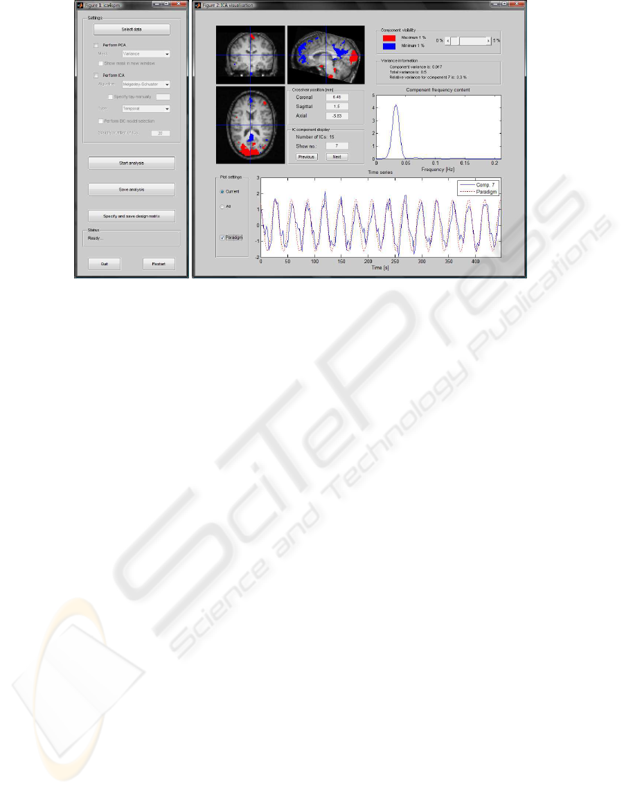
Figure 2: Left; The main user interface for the

ica4spm

toolbox. Right; Example of the ICA visualization user interface of

the

ica4spm

toolbox showing a temporal MS ICA component.

of the greatest/least intense voxels are superimposed.

In addition, it is possible to examine the temporal pat-

tern and frequency content of each IC and compare

that to a paradigm. If the user ﬁnds it relevant to in-

clude a given IC in the GLM, the toolbox facilitates

speciﬁcation and export of the IC for use in a sub-

sequent SPM analysis. Fig. 3 shows three selected

components from a temporal MS ICA performed on

the demonstration data set. The temporal proﬁle and

frequencycontents of the two ﬁrst componentsclearly

indicate that these components are related to the vi-

sual paradigm with a 30 second period and the spatial

map show activity restricted to the visual areas of the

brain. The analysis has split visual activity into two

components allowing it to capture activity regardless

of the phase. The last component shows how the ICA

has also captured nuisance signal variation related to

the cardiac cycle. Notice, that the temporal proﬁle of

this component appears aliased due the low sampling

rate. Figure 3 shows a test for signiﬁcant effects in the

test data set based on paradigm related ICs identiﬁed

in the training data set.

5 DISCUSSION & CONCLUSION

Our

ica4spm

toolbox facilitates easy unsupervised

exploratory analysis and visualization of relevant sig-

nal components from a data set and the use of ex-

tracted ICs in a SPM analysis. From the

ica4spm

main GUI, it is easy to load fMRI data and select

which settings to use for the ICA. If selected, PCA is

performed for dimensionality reduction of the data set

and BIC can be used to automatically for determin-

ing the number of relevant signal components. This

makes it easy to ensure that all relevant signal com-

ponents are discovered. The components of interest

can be saved to a design matrix and loaded in SPM5.

Generally, the use of structures in the program have

made it possible to access all data and variables at all

times.

ICA was found useful when applied to a real fMRI

data set, as it was able to identify both paradigm and

nuisance related effects. The activation related to the

paradigm was split into two components with differ-

ent phases in order to model any phase of the visual

stimuli. In subsequent SPM analysis with the time

series as regressors in the design matrix, we found

strong visual cortex as expected, see Fig. 3. Our

ﬁndings are equivalent to those found in (Lund et al.,

2006) for the same data set. Furthermore, it was pos-

sible to recognize ICs containing the pulse and res-

piration, making it possible to include these as con-

founding effects in the design matrix. In conclusion,

we found that the GUI may prove useful in the analy-

sis of fMRI data.

ACKNOWLEDGEMENTS

This work is supported by the Lundbeck Foundation

through the Center for Integrated Molecular Brain

Imaging (www.cimbi.dk).

BIOSIGNALS 2009 - International Conference on Bio-inspired Systems and Signal Processing

320

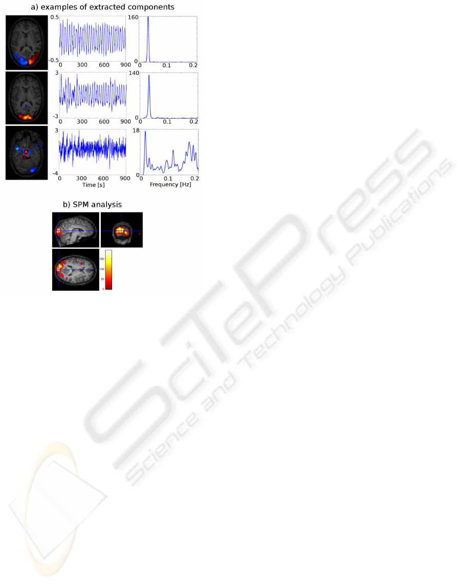
Figure 3: Top; Three selected components from ICA per-

formed on the demonstration dataset. To the left the spatial

map from each component is showed as an overlay on the

anatomical scan. For the ﬁrst two components a slice near

the calcarine sulcus is shown whereas a slice near the cir-

cle of Willis is shown for the last component. The middle

column of ﬁgures shows the temporal proﬁle for each of the

components and the right column shows the power spec-

trum (Welch method). The ﬁrst two components are clearly

related to the visual paradigm with prominent activity in the

occipital cortex whereas the last component is related to car-

diac nuisance effects. Buttom; F-test conducted in SPM5

on test data set for signiﬁcant effects of paradigm related

ICs identiﬁed in the training data set. Thresholded at p <

0.001 uncorrected.

REFERENCES

Bell, A. and Sejnowski, T. (1995). An information-

maximization approach to blind separation and blind

deconvolution. Neural Computation, 7:1129–1159.

Cardoso, J.-F. (1999). High-order contrasts for independent

component analysis. Neural Comput., 11(1):157–192.

Correa, N., Adali, T., and Calhoun, V. (2007). Performance

of blind source separation algorithms for fmri analy-

sis using a group ica method. Magnetic Resonance

Imaging, 25(5):684–694.

Frackowiak, R., Friston, K., Frith, C., Dolan, R., Price, C.,

Zeki, S., Ashburner, J., and Penny, W. (2003). Human

Brain Function. Academic Press, 2nd edition.

Hansen, L., Larsen, J., and Kolenda, T. (2001a). Blind de-

tection of independent dynamic components. Acous-

tics, Speech, and Signal Processing, 2001. Proceed-

ings. (ICASSP ’01). 2001 IEEE International Confer-

ence on, 5:3197–3200.

Hansen, L., Larsen, J., and Kolenda, T. (2001b). Blind de-

tection of independent dynamic components. Acous-

tics, Speech, and Signal Processing, 2001. Proceed-

ings.(ICASSP’01). 2001 IEEE International Confer-

ence on, 5.

Hansen, L., Larsen, J., Nielsen, F., Strother, S., Rostrup, E.,

Savoy, R., Lange, N., Sidtis, J., Svarer, C., and Paul-

son, O. (1999). Generalizable Patterns in Neuroimag-

ing: How Many Principal Components? Neuroimage,

9(5):534–544.

Højen-Sørensen, P., Winther, O., and Hansen, L. (2002).

Analysis of functional neuroimages using ICA adap-

tive binary sources. Neurocomputing, 49(1):213–225.

Hu, D., Yan, L., Liu, Y., Zhou, Z., Friston, K. J., Tan, C.,

and Wu, D. (2005). Uniﬁed spm-ica for fmri analysis.

NeuroImage, 25:746–755.

Hyv¨arinen, A. and Oja, E. (1997). A fast ﬁxed-point al-

gorithm for independent component analysis. Neural

Computation, 9(7):1483–1492.

Hyv¨arinen, A. and Oja, E. (2000). Independent component

analysis: Algorithms and applications. Neural Net-

works, 13(4-5):411–430.

Kolenda, T., Hansen, L., and Larsen, J. (2001). Signal

detection using ICA: Application to chat room topic

spotting. Third International Conference on Indepen-

dent Component Analysis and Blind Source Separa-

tion, pages 540–545.

Lund, T., Madsen, K., Sidaros, K., Luo, W., and Nichols,

T. (2006). Non-white noise in fMRI: Does modelling

have an impact? Neuroimage, 29(1):54–66.

McKeown, M., Hansen, L., and Sejnowsk, T. (2003a). Inde-

pendent component analysis of functional MRI: what

is signal and what is noise? Current Opinion in Neu-

robiology, 13(5):620–629.

McKeown, M., Hansen, L., and Sejnowsk, T. (2003b). Inde-

pendent component analysis of functional mri: what is

signal and what is noise? Current Opinion in Neuro-

biology, 13(5):620–629.

McKeown, M., Makeig, S., Brown, G., Jung, T., Kinder-

mann, S., Bell, A., and Sejnowski, T. (1998). Analysis

of fmri data by blind separation into independent spa-

tial components. Human Brain Mapping, 6(5):160–

188.

Molgedey, L. and Schuster, H. (1994). Separation of

independent signals using time-delayed correlations.

Physical Review Letters, 72(23):3634–3637.

Smith, L. (2002). A tutorial on Principal Components Ana-

lysis. Cornell University, USA, 51:52.

UNIFIED ICA-SPM ANALYSIS OF FMRI EXPERIMENTS - Implementation of an ICA Graphical User Interface for the

SPM Pipeline

321