
ON THE INFLUENCE OF LOW FREQUENCY COMPONENTS IN
THE WEIGHT BEHAVIOUR OF THE LMS ALGORITHM
D. S. Brito, R. C. S. Freire
Department of Electrical Engineering, Federal University of Campina Grande
Rua Aprigio Veloso, 882, 58.109-900 - Campina Grande - PB, Brazil
E. Aguiar, F. Lucena, A. K. Barros
Department of Electrical Engineering, Federal University of Maranhao
Avenida dos Portugueses, S/N, 65080-040 - Sao Luis - MA - Brazil
Keywords:
Adaptive algorithms, LMS algorithm, ECG, LMS spectrum, Low frequency, Very low frequency.
Abstract:
The Least Mean Square (LMS) algorithm is a very important tool in the estimation and filtering of biomedical
signals. Amongst these signals are the periodic and quasiperiodic. For example, the LMS algorithm was used
to estimate the coefficients of the Fourier series at a given frequency or even in a spectral analysis. In this
paper we study the behavior of the weights of the LMS algorithm when the signal to be estimated acts at very
low frequencies. We prove theoretically that lower frequency noise affects the estimation of the weights at
higher frequencies. We carried out simulations and showed that experimental findings are in agreement with
the theoretical results. Moreover, we exemplify the problem with electrocardiogram signals (ECG).
1 INTRODUCTION
Quasiperiodic physiological signals such as the
electrocardiogram (ECG) are susceptible to various
interferences. According to (Friesen et al.,
1990), the main sources of noises and artifacts
in ECG signal are: power line interference,
electrode contact noise, motion artifacts, muscle
contraction (electromyographic, EMG), baseline drift
and ECG amplitude modulation with respiration,
instrumentation noise generated by electronic devices
used in signal processing, electrosurgical noise and
impedance cardiography signals (ZCG). Some of
those interference signals have low frequency (0.04–
0.15 Hz) and very low frequency (0.0033–0.04 Hz)
components, that influence on the acquisition and
analysis of the ECG signal.
In figure 1, we show the power spectrum of an
ECG signal under the influence of low and very low
frequencies. Analyzing its spectrum it is possible
to ascertain the disturbances at low and very low
frequencies. These kind of noises may interfere in
the analysis of the signal.
Many solutions to filter general disturbances on
biological signals have been proposed. Amongst
them there are those which use adaptive methods,
such as the Fourier Linear Combiner (FLC) proposed
by (Vaz and Thakor, 1989), (Vaz et al., 1994). After
that, it was suggested the Scaled FLC (SFLC) in
(Barros et al., 1995) to eliminate not only non-
correlated noises but also body movements (Barros
and Ohnishi, 1997). It is important to emphasize that
the FLC is used as spectrum analyzer as proposed
by Widrow (Widrow et al., 1987). In this method,
the reference inputs are sinusoidal and co-sinusoidal
functions and the LMS algorithm (Widrow and
Hoff Jr., 1960) is used to estimated the coefficients
of a Fourier series in (Widrow et al., 1976), (Widrow
and Stearns, 1985).
In this work we used the FLC to estimate the
spectrum of biomedical signals, specifically ECG
signals in the presence of low or very low frequency
noise, and studied the behavior of the weights
estimated by the LMS algorithm. We show that if
there is a constant component or even a low frequency
noise added to the desired signal, the behavior of the
weights of the LMS algorithm will be changed.
This work is organized as follows. In section 1
we describe the problem present a brief introduction
on the topic. In 2 we make the problem demonstration
345
S. Brito D., C. S. Freire R., Aguiar E., Lucena F. and K. Barros A. (2009).
ON THE INFLUENCE OF LOW FREQUENCY COMPONENTS IN THE WEIGHT BEHAVIOUR OF THE LMS ALGORITHM.
In Proceedings of the International Conference on Bio-inspired Systems and Signal Processing, pages 345-350
DOI: 10.5220/0001550803450350
Copyright
c
SciTePress
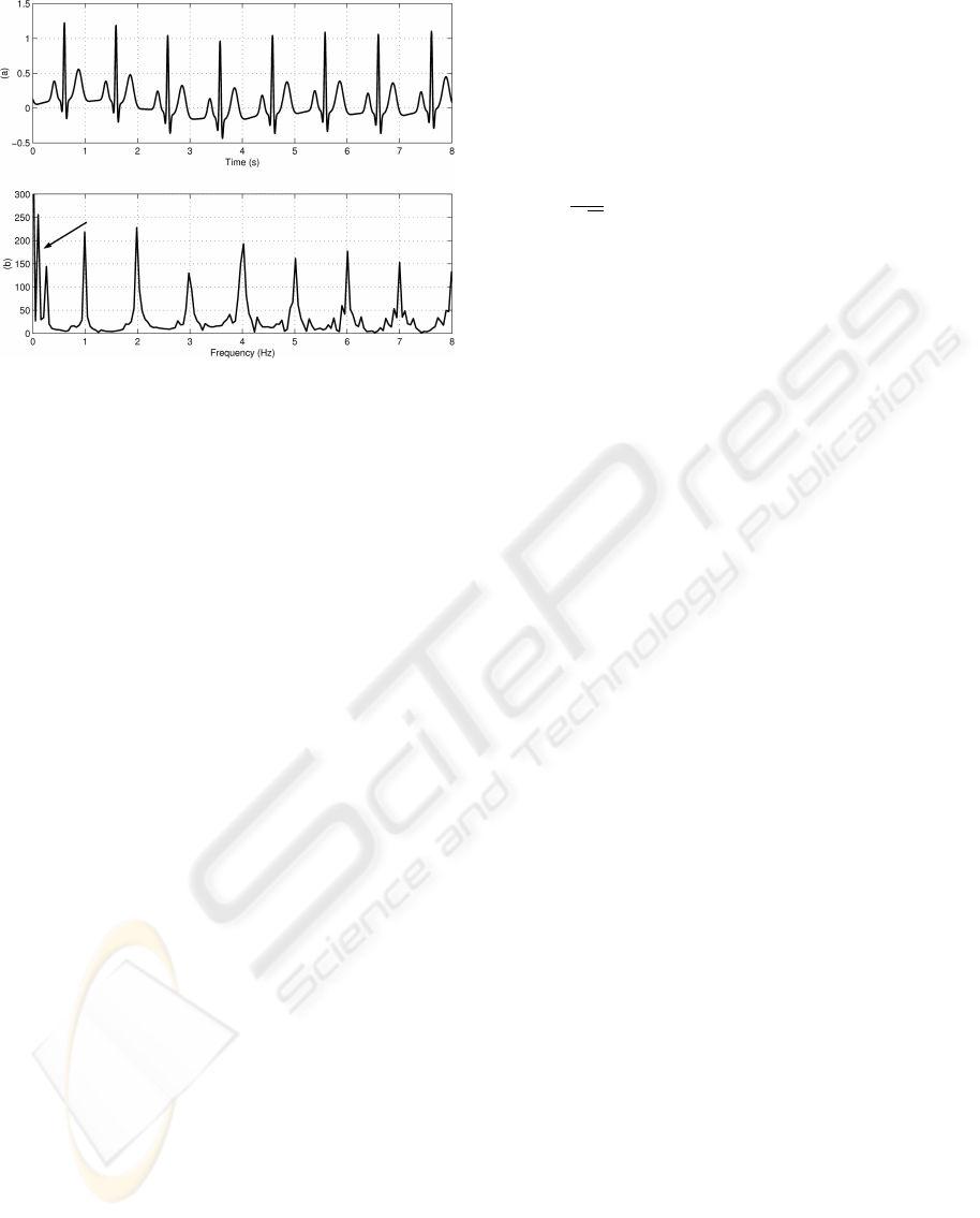
Figure 1: The spectrum response of a signal
electrocardiogram (ECG) synthetic. In (a) we have
an ECG synthetic signal and (b) its Fast Fourier Transform
(FFT).
describe the methods used in our analysis. In section 3
we show the results obtained in simulations and the
applications of the method. Finally in sections 4 and 5
we make comments to improve the understanding of
the work and the conclusion respectively.
2 METHODS
Our method was developed by implementing the
Fourier linear combiner (FLC) according to the block
diagram on figure 2. The LMS algorithm is used
to estimate the coefficients of the Fourier series.
This method is known as LMS spectrum analyzer.
The reference inputs are pairs of sines and co-sines.
We propose the LMS spectrum estimation for a
given frequency band and suppose that these low
frequency noises affects the spectrum estimation of
ECG signals.
2.1 Periodic and Quasiperiodic Signals
A periodic or quasiperiodic signal can be expressed
as a combination of Fourier series and therefore can
be reconstructed as:
s
k
=
l
∑
n=1
A
nk
sin(c
n
ω
0
k) +
l
∑
n=1
B
nk
cos(c
n
ω
0
k), (1)
where ω
0
is the fundamental frequency and c
n
=
[c
1
, ··· , c
l
] is a vector defining the frequency band.
c
1
ω
0
is lowest estimated frequency components and
c
l
ω
0
the highest. k is the discrete time index and
A
nk
and B
nk
time variant Fourier series coefficients.
The variations on these coefficients occur due to the
quasiperiodic nature of the signal, which means that
the fundamental frequency of the signal, together with
the harmonics, have little variation along time.
To estimate the coefficients A
nk
and B
nk
we used
adaptive linear combiner (ALC), developed by (Vaz
et al., 1994). The reference input vectors, X
k
, is
defined as,
X
k
=
1
√
N
[sin(c
n
ω
0
k) ··· cos(c
n
ω
0
k) ···]
H
, (2)
where N correspond to the number of harmonic and
H is the Hermitian operator.
2.2 LMS Algorithm
We used the LMS algorithm as a spectrum analyzer
as employed by Widrow (Widrow et al., 1987), in
which he discussed the relationship between the DFT
(Discrete Fourier Transform) and the vector weight
W
k
estimated by the algorithm. This algorithm
calculates the possible variations in time which result
in an instantaneous output, y
k
, which is given by
the internal product between the reference inputs X
k
and the vector weight W
k
. Mathematically this is
presented as follows,
y
k
= X
H
k
W
k
= W
H
k
X
k
, (3)
where W
k
is composed of updated weights
[w
1k
, w
2k
, ··· , w
lk
]. The initial weight vector
was set to zero, as used by Widrow et al. in (Widrow
et al., 1987). Consider a noise ν
k
, inherent to the
acquisition process of the desired signal, which is
non-correlated to ECG signal.
The weights of the adaptive system are adjusted or
updated by steepest descent method, as described by
Widrow in (Widrow and Stearns, 1985). The output
of the LMS algorithm y
k
, is subtracted from the signal
d
k
, which is corrupted by noises generating an error
ε
k
, which we want to minimize to obtain the LMS
spectrum.
2.3 Weight Behavior
In this section we demonstrate that low frequency
disturbances present on ECG signal interfere on the
estimation of LMS spectrum. We consider low and
very low noises as being those disturbances below the
fundamental frequency of the signal.
We start this analysis from the adaptation rule of
the LMS algorithm (Widrow and Hoff Jr., 1960):
W
k+1
= W
k
+ 2µε
k
X
k
, (4)
where µ is a real positive number which represents
the size of the step or learning rate and controls the
BIOSIGNALS 2009 - International Conference on Bio-inspired Systems and Signal Processing
346
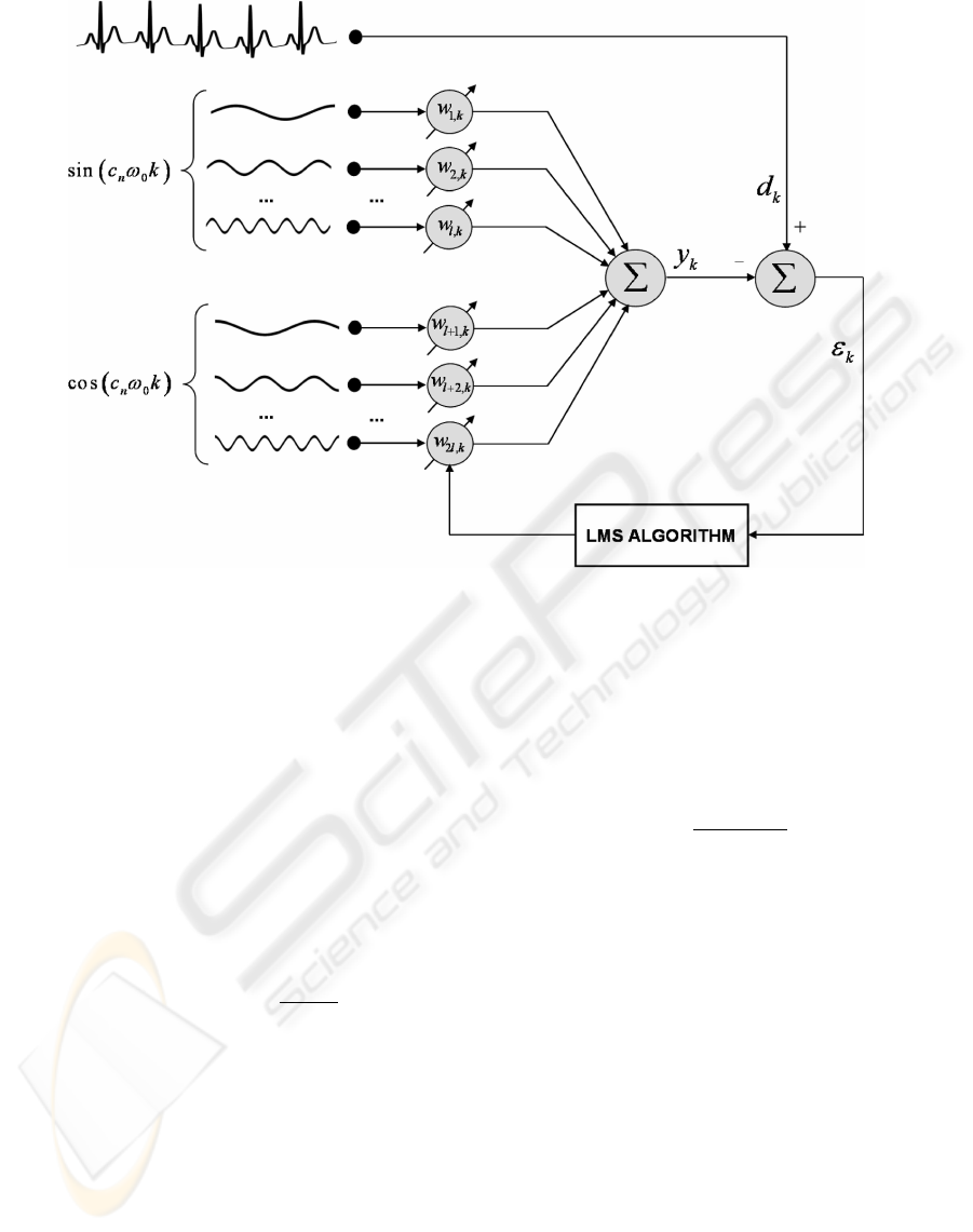
Figure 2: Block diagram of the Fourier Linear Combiner and of the LMS algorithm implemented. d
k
is a synthesized ECG
signal add ν
k
a very low frequency noise inherent the acquisition.
x
1,k
, x
2,k
, ···x
l,K
T
is the vector of reference inputs,
composed by pairs of sines and cosines and ε
k
is the error given by ε
k
= d
k
−y
k
.
system stability. Let us define the error ε
k
= d
k
−y
k
and the signal d
k
= s
k
+ ν
k
in which s
k
is the desired
signal and ν
k
is the additive low frequency noise.
Substituting ε
k
in equation (4), the updated
weights become,
W
k+1
= W
k
+ 2µ
s
k
X
k
+ ν
k
X
k
−X
H
k
W
k
X
k
, (5)
Applying the expected to the value updated
weights in equation (5) and doing appropriate
considerations (appendix) we obtain the following
result,
E [W
k
] = 2µDx
0
E
h
D
−k
i
E [ν
k−1
]
1 −
˜
H
k
1 −
˜
H
+ W
∗
, (6)
where W
∗
is the optimal weight.
The term E
D
−k
E [ν
k−1
] is sinusoidally time
variant for it is non-stationary and its expected value
changes through time, therefore we call sinusoidal
perturbation factor (SPF).
As proposed by Widrow (Widrow et al., 1987)
a learning rate equal to 0.5 estimates exactly the
DFT of the signal, but lower learning rates can be
used to estimate the signal (Barros et al., 1995), and
therefore sufficient to make an approximation of the
LMS spectrum.
For periodic signals, the coefficients of the series
are not time variant. However, in the case of the quasi
periodic signals, the behavior of the coefficients of the
Fourier series is time variant, since the period of the
signal cycles is not constant.
The magnitude of each frequency component can
be obtained by
C
n,k
=
q
A
2
n,k
+ B
2
n,k
, (7)
where A
n,k
= W
n,k
and B
n,k
= W
n+N,k
. With those
weights we estimate a spectrogram or LMS spectrum.
The spectrogram is a graph that represents the signal
power, simultaneously in the time and frequency
domains in each instant.
3 RESULTS
The adaptive system was implemented as illustrated
in figure 2. In the first experiments we used a 1.2 Hz
sinusoidal signal as d
k
and 0.01 Hz additive sinusoidal
noise. The frequency band of the reference inputs was
in the range 1.0 Hz to 1.5 Hz, in steps of 0.05 Hz,
giving a number of 11 harmonics.
To verify the effect of the low frequency
disturbance, as observed on equation (6), we
eliminated the low frequency noise using a high-
pass, 4
th
order, butterworth digital filter with 0.50
ON THE INFLUENCE OF LOW FREQUENCY COMPONENTS IN THE WEIGHT BEHAVIOUR OF THE LMS
ALGORITHM
347

Figure 3: LMS spectrum for a theoretical simulated signal.
In (a) we show the LMS spectrum of a sinusoidal signal
with frequency of 1.2 Hz with a low frequency additive
sinusoidal noise of 0.01 Hz. In (b) the spectrum of
the filtered sinusoidal signal and in (c) the error between
spectra.
Hz cutoff frequency. In figure 3 we present the
LMS spectrum for the simulated theoretical noise
sinusoidal signal and the filtered version signal. We
also accomplished some experiments with real and
synthesized biomedical signals. The synthesized
ECG signal was created with an inherent low
frequency noise, and it is supposed to approximate
an ECG signal from a resting subject generated by
ECGSYN program of the PhysioNet (Goldberger
et al., e 13). For the ECG signal the frequency range
of the reference inputs was 0.5 Hz to 1.5 Hz, which
is in general sufficient to estimate the fundamental
frequency.
In figure 4 we show the LMS spectrum obtained
and the spectral error by the estimation of the
synthesized ECG signal and its filtered version using
the same filtering process of the previous test. To
validate this result, we also accomplished simulation
with real biomedical signals, specifically an ECG
signal of normal patients. In figure 5 we show the
LMS spectrum of the noise signals high-pass filtered.
4 DISCUSSIONS
Observing figure 3, we can say that low frequency
noises affect the estimation of the spectrum signal
when we use the LMS algorithm as a spectrum
analyzer. In figure 3a, we verify, starting from the
LMS spectrum, the sinusoidal influence along time
as a ripple effect in the fundamental frequency, as
well as on the other harmonic frequency components.
These results corroborate the theoretical calculations
that culminate in the equation (6).
Figure 4: LMS spectrum of an ECG synthesized signal
simulating resting conditions. In (a) we show that
the spectrum is influenced by the low frequency noises
originated of the movement artifacts, breathing etc. In (b)
we show the LMS spectrum of the high-pass filtered ECG
signal and in (c) the error between spectra.
Figure 5: LMS spectrum of real ECG signal from a patient
at rest. In (a) we show that the LMS spectrum is influenced
by the low frequency noise. In (b) we show the LMS
spectrum filtered by high-pass butterworth filter and in (c)
the error between spectra.
Examining the equation (6), it can be observed
that the expected value of the weights is composed of
two terms. The term on the left is the expected value
of the weight while the first term on the right side
varies sinusoidally in time as a function of the term
E [ν
k−1
]. When the expected value of the noise term
is equal to zero, the term for the whole equation will
also be zero, since it is multiplied by all of the other
variables. The expected value of the weight being
equal to the optimum weight is a consequence of the
absence of any non-stationary noise into the signal,
specifically a noise whose expected value changes in
time (ideal condition); or yet when the noise ν
k
is in a
higher frequency band; then its expected value is also
BIOSIGNALS 2009 - International Conference on Bio-inspired Systems and Signal Processing
348

zero. This way, LMS spectrum estimation of ECG
signal becomes susceptible to movement artifacts,
breathing noise and electromyography signal which
are low and very low frequency noises. In fact for the
theoretical signal test the fundamental frequency of
the desired signal is 1.2 Hz, while the noise was 0.01
Hz. The relationship is only 120 times higher.
In figure 3b, we present an estimation of
the filtered sinusoidal signal to eliminate the low
frequency noises. Observing the LMS spectrum we
can see that there is no sinusoidal influence on the
spectrum, as expected, since the low frequency noise
was eliminated from the signal. Then we have a most
precise spectral estimation being constant through
time. In figure 3c we represent the error between LMS
spectrum of the noise signal and the filtered signal.
Since the influence of the noise in the spectrum is
sinusoidal, which can be eliminated by filtering the
signal, the error is also sinusoidal.
In figure 4 and 5, we presented the LMS spectrum
of biomedical synthesized ECG signal and a real
ECG, respectively. Observing figure 4a and 5a, we
note a strong sinusoidal influence in the fundamental
frequency and along the first harmonic. In figure 4b
and 5b, respectively, we have the LMS spectrum
of the filtered signal. Therefore we observe the
absence of the low frequencies interference in the
LMS spectrum. It is practically constant in the
fundamental frequency of the signal. In figure 4c and
5c we observe the some pattern of error present in the
figure 3c.
5 CONCLUSIONS
We have demonstrated theoretically and through
simulations that, using the LMS algorithm as
a spectrum analyzer of biomedical signals, the
estimated weights are sinusoidally affected by low
frequency noises. In general, biomedical signals,
such as ECG, EMG and ZCG, are acquired along
with low frequency noises, due to body movements,
respiration and other less significant noise sources.
This implies that we should be concerned with this
type of estimation.
ACKNOWLEDGEMENTS
The authors would like to thank the Foundation
of Support to the Research and the Scientific and
Technological Development of the Maranhao State
(FAPEMA) for the grants given, to the Maranhao
State Education Secretary (SEDUC-MA) and the Sao
Luis City Department of Education (SEMED), for
financing the studies. We also thank CNPq and Capes
for financial support for the project. The authors are
also grateful for the contributions of Ewaldo Eder
Junior and Denner Guilhon by revision.
REFERENCES
Barros, A. K. and Ohnishi, N. (1997). Mse behavior of
biomedical event-related filters. IEEE Transactions
Biomedical Engineering, BME-44(9):848–855.
Barros, A. K., Yoshizawa, M., and Yasuda, Y. (1995).
Filtering non-correlated noise in impedance
cardiography. IEEE Transactions on Biomedical
Engineering, 42(3):324–327.
Friesen, G., Jannett, T., Jadallah, M., Yates, S., Quint, S. R.,
and Nagle, H. (1990). A comparison of the noise
sensitivity of nine qrs detection algorithms. IEEE
Transactions on Biomedical Engineering, 37(1):85–
98.
Goldberger, A. L., Amaral, L. A. N., Glass, L., Hausdorff,
J. M., Ivanov, P. C., Mark, R. G., Mietus, J. E.,
Moody, G. B., Peng, C.-K., and Stanley, H. E. (2000
June 13). PhysioBank, PhysioToolkit, and PhysioNet:
Components of a new research resource for complex
physiologic signals. Circulation, 101(23):e215–
e220. Circulation Electronic Pages: http://
circ.ahajournals.org/cgi/content/full/101/23/e215.
Vaz, C. A., Kong, X., and Thakor, N. V. (1994). An adaptive
estimation of periodic signals using a fourier linear
combiner. IEEE Transactions on Signal Processing,
42(1):1–10.
Vaz, C. A. and Thakor, N. V. (1989). Adaptive fourier
estimation of time-varying evoked potentials. IEEE
Transactions Biomedical Engineering, 36(4):448–
455.
Widrow, B., Baudrenghien, P., Vetterli, M., and Titchener,
P. (1987). Fundamental relations between the lms
algorithm and dft. IEEE Transactions on Circuits and
Systems, 7(Cas-34):814–820.
Widrow, B. and Hoff Jr., M. E. T. (1960). Adaptive
switching circuits. In Proceedings IRE WESCON
Convention Record, pages 96–104, New York.
INSTICC Press.
Widrow, B., McCool, J. M., Larimore, M. G., and
Johnson Jr., C. R. (1976). Stationary and non-
stationary learning characteristics of the lms adaptive
filter. In Procedings IRE WESCON Convention
Record, pages 1151–1162. I Proc. of the IEEE.
Widrow, B. and Stearns, S. D. (1985). Adaptive Signal
Processing. Prentice-Hall Signal Processing Series,
New Jersey - USA, 1st. edition.
ON THE INFLUENCE OF LOW FREQUENCY COMPONENTS IN THE WEIGHT BEHAVIOUR OF THE LMS
ALGORITHM
349

APPENDIX
We begin the demonstration starting from the
expression that represents the updated weight vector
given by,
W
k+1
= W
k
+ 2µε
k
X
k
, (A1)
where µ is a positive real number representing the
step size or the learning rate, while determines and
controls the system’s stability, and ε
k
is the error
defined by ε
k
= d
k
− y
k
, with d
k
defined by d
k
=
s
k
+ν
k
, where s
k
is a desired signal and ν
k
is the added
undesirable signal as it can be observed in figure 2.
Substituting ε
k
in equation (A1), the updated
weights become,
W
k+1
= W
k
+ 2µε
k
X
k
W
k+1
= W
k
+ 2µ
d
k
−X
H
k
W
k
X
k
W
k+1
= W
k
+ 2µ(s
k
X
k
+ ν
k
X
k
−X
H
k
W
k
X
k
),
(A2)
By expressing ε
k
in terms of statistical error
estimation parameters, equation (A2) becomes,
W
k+1
= W
k
+ 2µX
k
X
H
k
W
∗
+ ν
k
−X
H
k
W
k
W
k+1
−W
∗
= W
k
−W
∗
+ 2µX
k
ν
k
−2µX
k
X
H
k
(W
k
−W
∗
), (A3)
Replacing W
k+1
−W
∗
by
˜
W
k+1
and W
k
−W
∗
by
˜
W
k
we get an equation for the system weight, given
by,
˜
W
k+1
=
I −2µX
k
X
H
k
˜
W
k
+ 2µX
k
ν
k
, (A4)
Let us define a 2N x 2N diagonal matrix D
with diagonal elements, D(q, q) = D
q
= e
jω
0
q
, q =
−N, −(N −1), . . . , −1, 1, . . . , N and X
0
=
2N times
z }| {
[1, 1, . . . , 1]
T
. The new inputs X
k
will be expressed
by X
k
= D
−k
X
0
and its conjugate X
∗
k
= D
k
X
0
.
Multiplying both sides of equation (A4) by D
k+1
,
we have
D
k+1
˜
W
k+1
= D
k+1
˜
W
k
−2µD
k+1
D
−k
X
0
X
T ∗
0
D
k
˜
W
k
+2µD
k+1
D
−k
X
0
ν
k
D
k+1
˜
W
k+1
= D
I −2µX
0
X
T
0
D
k
˜
W
k
+2µDX
0
ν
k
, (A5)
Making
˜
V
k
= D
k
˜
W
k
,
˜
H = D
I −2µX
0
X
T
0
,
˜
V
k+1
= D
k+1
˜
W
k+1
and replacing them in equation
(A5), we can re-written as,
˜
V
k+1
=
˜
H
˜
V
k
+ 2µDX
0
ν
k
, (A6)
Assuming that D
k
and W
k
are statistically
independent, thus the value expected of equation (A6)
can be re-written as,
E
˜
V
k+1
= E
˜
H
˜
V
k
+ 2µE [DX
0
ν
k
], (A7)
Once D and X
0
are invariant in time,
equation (A7) will become,
E
˜
V
k+1
= 2µDX
0
E [ν
k
]
k
∑
i=1
˜
H
i
+(2µDX
0
E [ν
k
])
n
, (A8)
Making n >> 1, then µ
n
→0, thus the second term
of the right side of the equation (A8) is null, once
0 < µ < 1. Expanding the very same equation (A8)
into a geometric series, then we attain,
E
h
D
k
i
E
˜
W
k
= 2µDX
0
E [ν
k−1
]
1 −
˜
H
k
1 −
˜
H
, (A9)
Returning back to former variables and
multiplying equation (A9) by E[D
−k
], making
˜
W
k
= W
k
−W
∗
we get
E [W
k
−W
∗
] = 2µDX
0
E
h
D
−k
i
E [ν
k−1
]
1 −
˜
H
k
1 −
˜
H
,
(A10)
As W
∗
is the optimal weight which is an arbitrary
constant, then we can express this result, by
E [W
k
] = 2µDX
0
E
h
D
−k
i
E [ν
k−1
]
1 −
˜
H
k
1 −
˜
H
+ W
∗
.
(A11)
where E
D
−k
E [ν
k−1
] is a time variant term that we
call sinusoidal perturbation factor (SPF).
BIOSIGNALS 2009 - International Conference on Bio-inspired Systems and Signal Processing
350
