BAYESIAN SCENE SEGMENTATION INCORPORATING MOTION

CONSTRAINTS AND CATEGORY-SPECIFIC INFORMATION

Alexander Bachmann and Irina Lulcheva

Department for Measurement and Control, University of Karlsruhe (TH), 76 131 Karlsruhe, Germany

Keywords:

Stereo vision, Motion segmentation, Markov Random ﬁelds, Object classiﬁcation, Global image context.

Abstract:

In this paper we address the problem of detecting objects form a moving camera by jointly considering low-

level image features and high-level object information. The proposed method partitions an image sequence

into independently moving regions with similar 3-dimensional (3D) motion and distance to the observer. In the

recognition stage category-speciﬁc information is integrated into the partitioning process. An object category

is represented by a set of descriptors expressing the local appearance of salient object parts. To account for the

geometric relationships among object parts a structural prior over part conﬁgurations is designed. This prior

structure expresses the spatial dependencies of object parts observed in a training data set. To achieve global

consistency in the recognition process, information about the scene is extracted from the entire image based

on a set of global image features. These features are used to predict the scene context of the image from which

characteristic spatial distributions and properties of an object category are derived. The scene context helps to

resolve local ambiguities and achieves locally and globally consistent image segmentation. Our expectations

on spatial continuity of objects are expressed in a Markov Random Field (MRF) model. Segmentation results

are presented based on real image sequences.

1 INTRODUCTION

One of the cornerstones in the development of auto-

motive driver assistance systems is the comprehen-

sive perception and understanding of the environment

in the vicinity of the vehicle. Especially for appli-

cations in the road trafﬁc domain the robust and re-

liable detection of close-by trafﬁc participants is of

major interest. In this context, vision sensors pro-

vide a rich and versatile source of information (Sivak,

1996), (Rockwell, 1972). Visual object detectors are

expected to cope with a wide range of intra-class char-

acteristics, i.e. variations in the visual appearance of

an object due to changes in orientation, lighting con-

ditions, scale, etc.. At the same time, these methods

must retain enough speciﬁcity to yield a minimum

amount of misclassiﬁcations. Here, most of the ap-

proaches developed in the last decades can be parti-

tioned into either: (i) methods based on classiﬁcation

which constrain the detection process to a very spe-

ciﬁc representation of an object learned from a ref-

erence data set or (ii) methods performing object de-

tection by employing local object characteristics on

a low level of abstraction using image-based criteria

to describe coherent groups of image points as e.g.

grey level similarity, texture or motion uniformity of

image regions. A major drawback of these meth-

ods is the fact that the grouping criteria mostly ig-

nore object-speciﬁc properties with the consequence

of misdetection rates in cluttered real world scenes

that are still prohibitive for most driver assistance ap-

plications. This limitation can be weakened by clas-

siﬁcation methods that have proven to detect a large

portion of typical objects at moderate computational

cost.

In our approach object detection is performed

based on the relative motion of textured objects and

the observer. The expectation of spatial compactness

for most real world objects is expressed by its posi-

tion relative to the observer. To obtain a dense rep-

resentation of the observed scene, object detection is

formulated as an image segmentation task. Here, each

image point is tested for consistency with a set of pos-

sible hypothesis, each deﬁned by a 3D motion and po-

sition. The set of object parameters that best explains

the measured quantities of the image point is assigned

to the image point.

To further increase the quality of the segmenta-

291

Bachmann A. and Lulcheva I. (2009).

BAYESIAN SCENE SEGMENTATION INCORPORATING MOTION CONSTRAINTS AND CATEGORY-SPECIFIC INFORMATION.

In Proceedings of the Fourth International Conference on Computer Vision Theory and Applications, pages 291-298

DOI: 10.5220/0001653302910298

 SciTePress

tion result, we incorporate information about the ob-

jects to be recognised by the system. The integra-

tion of object-speciﬁc information for driving image

segmentation methods has recently developed into a

ﬁeld of active research and seems to be a promis-

ing way to incorporate more information into exist-

ing low-level object detection methods, see e.g. (Ohm

and Ma, 1997; Burl et al., 1998). Our work is in-

spired by recent research results in human vision,

as e.g. (Rentschler et al., 2004), indicating that the

recognition and segmentation of a scene is a heavily

interweaved process in human perception. Follow-

ing this biological model our segmentation method

is based on low-level features but guided and sup-

ported by category-speciﬁc information. The ques-

tion of how to describe this knowledge is very chal-

lenging because there is no formal deﬁnition of what

constitutes an object category. Though most people

agree on the choice of a certain object category, there

is still much discussion on the choice of an appropri-

ate object descriptor. In our approach the high-level

information comprises the appearance of a set of char-

acteristic object parts and its arrangement relative to

each other and in the scene. Though good for model-

ing local object information it fails to capture global

consistency in the recognition process, as e.g. the de-

tection of a car in a tree high above the road. We

establish global consistency by exploiting the close

relationships of certain object categories to the scene

of the image. The method characterises a scene by

global image features and derives the predicted cat-

egory likelihood and distribution of an object for a

particular scene. We argue that the incorporation of

category-speciﬁc scene context into our scene seg-

mentation framework can drastically improvethe pro-

cess as (i) insufﬁcient intrinsic object information can

be augmented with and (ii) local ambiguities can be

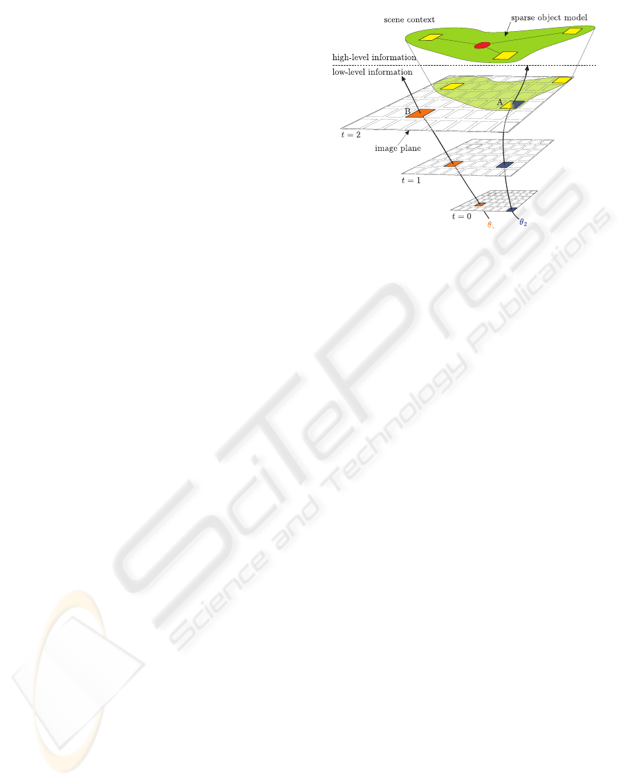
better resolved from a global perspective. Figure 1

shows the principle of our probabilistic image seg-

mentation framework.

The remainder of the paper is organised as fol-

lows. Section 2 recalls some of the theoretical back-

ground that is needed to understand image segmen-

tation as presented here. It is shown how object-

speciﬁc information can be incorporated into the ex-

isting probabilistic framework by means of a sparse

object model and category-speciﬁc scene informa-

tion. Section 3 presents the experimental results be-

fore conclusions are drawn in Section 4.

Figure 1: Principle of the combined segmentation process.

Image segmentation is performed by a Bayesian maximum

a posteriori estimator assigning the most probable object

hypothesis to each image point. In the example, image

points are assigned to either object hypothesis 1 (B, ex-

pressed by θ

) or object hypothesis 2 (A, expressed by θ

2 SCENE SEGMENTATION

USING MRFs

This section outlines the mechanism that evaluates the

local and global properties of image points and sepa-

rates the image accordingly. Notably there are two

issues to be addressed in this task: (i) how to encour-

age the segmentation to consider local properties in

the image on a low abstraction level and (ii) how to

enforce the process to incorporate category-speciﬁc

information into the segregation of the image.

First, a number of constraints are formulated that

specify an acceptable solution to the problem. In

computer vision, commonly the data and prior knowl-

edge are used as constraints. The data constraint re-

stricts a desired solution to be close to the observed

data and the prior constraint conﬁnes the desired solu-

tion to have a form agreeable with the a priori knowl-

edge.

The challenging task is the estimation of object

parameters θ =



, .., θ



given an observation set

Y which has been generated by an unknown and con-

stantly changing number of objects K. Within our

framework we solved this by formally expressing the

scene segmentation process as labeling problem: Let

a set of sites (or units) P = {p

, .., p

} ,p

∈ R

and a

set of possible labels L be given with one label l

for

each site p

specifying the process which generated

the data. l

is a binary vector such that l

= 1 if object

j generated the data at site p

. The desired labeling

is then a mapping l : P 7→ L that assigns a unique la-

VISAPP 2009 - International Conference on Computer Vision Theory and Applications

292

bel to each site. The labeling l = (l(p

), .., l(p

)) =

, .., l

) shall ascertain that (i) the data of all sites

with identical label exhibit similarity w.r.t. some mea-

sure and that (ii) the labeling conforms with the a pri-

ori knowledge.

Taking a Bayesian perspective the posterior prob-

ability of a labeling l can be formulated

P(l|Y, θ) =

P(Y|l, θ)P(l|θ)

P(Y, θ)

, (1)

where we try to ﬁnd the labeling l which maximises

P(l|Y, θ). Here, P(Y|l, θ) states the data constraint

parametrised by object parameter vector θ. P(l|θ)

states the prior term. Obviously, P(Y) in Equation (1)

does not depend on the labeling l and can thus be

discarded during the maximization. By rearranging

Equation (1) the maximum a posteriori (MAP) esti-

mate of a labeling can be expressed

l = argmax

P(Y|l, θ)

| {z }

data term

P(l|θ)

|{z}

prior term

(2)

Assuming the observations Y to be i.i.d. normal,

the ﬁrst term in Equation (2) can be written

P(Y|l, θ) =

∏

i=1

P(y

, θ)

∝

∏

i=1

exp(−E

, θ)).

(3)

denotes an energy functional, rating observation y

given label vector l

and object parameter vector θ.

If there exists no prior knowledge about the val-

ues of θ (i.e. P(θ) = const.) prior expectations on l

can be modelled using MRFs. An MRF is deﬁned

by the property P(l

, .., l

i−1

, l

i+1

, l

) = P(l

, ∀

∈

), with G

being the neighbourhood set of image

point p

. The system must fulﬁll the constraints (i)

6∈ G

∀l

, no site is its own neighbour and (ii) p

∈

⇔ p

∈ G

, if p

is a neighbour of p

, then p

is also

a neighbour of p

. Due to the equivalence of MRF

and Gibbs distributions, see e.g. (Besag, 1974), an

MRF may be written as P(l) =

exp(−V

(l)), where

(l) ∈ R is referred to as clique potential which only

depends on those labels of l whose sites are elements

of clique k. A clique k ⊆ P is any set of sites such

that any of its pairs are neighbours. We model the

clique potential for 2-element cliques k =



, p



with |p

− p

| = 1 using an extension of the gener-

alised Potts model ((Geman and Geman, 1984))

{i, j}

, l

) =



λ if l

6= l

0 otherwise

, (4)

favoring identical labels at neighbouring sites. The

coefﬁcient λ modulates the effect of the prior term

and therefore the degree of label smoothness in the

segmentation result. The generalised Potts model is

a natural and simple way to deﬁne a clique poten-

tial function that describes the smoothness of neigh-

bouring points. With Equation (3)–(4), Equation (2)

evolves to

l = argmin

∑

i=1

, θ) +

∑

i=1

∑

j∈k

{

i, j}

, l

)

=argmin

Ψ(E, l, θ) .

(5)

2.1 Low-level Information

Concerning the data term, in (Bachmann and Dang,

2008) excellent results have been achieved using the

property object motion. Here, objects are speciﬁed by

a 6-degree-of-freedom(dof) parametric motion model

representing the motion of an image region by pa-

rameter vector v. The similarity between expected

and observed object motion is expressed by evalu-

ating the similarity between expected image texture

t−1

;r;v) derived from motion proﬁle v and ob-

served image texture G

;r) within a block of size

B centered around image point p

(ε

, v) =

∑

r∈B



;r) − G

t−1

;r;v)



, (6)

with ε

stating the residual at image position p

This object model has been further extended by

the object position ξ relative to the own vehicle, i.e.

θ = (v, ξ). The relative object position is expressed

by the mean disparity ξ

∆

of all image points assigned

to the respective label and the assignment energy of

image point p

given an object label is

(ε

, ξ) =



∆

− ξ

∆



2σ

∆

. (7)

∆

states the extension of the object in terms of the

variance of the disparity values assigned to the object

label.

The object model presented above allows to seg-

regate an image sequence into K distinct regions with

each region being deﬁned as homogenously moving

object at a certain distance to the observer, i.e. L =

{

background

object 2

, ..,

object K

}, with image

regions moving static relative to the observer (as e.g.

trees, buildings, etc.) being labeled {

background

With the intention to classify every image point

into a meaningful semantic category and due to the

well-known limitations of motion-based segmenta-

tion methods (as e.g. the aperture problem or poorly

textured image regions) the next step is to incorpo-

rate category-speciﬁc information into the segmenta-

tion process.

BAYESIAN SCENE SEGMENTATION INCORPORATING MOTION CONSTRAINTS AND CATEGORY-SPECIFIC

INFORMATION

293

2.2 Category-speciﬁc Information

Therefore we extend our algorithm to perform in-

terleaved object recognition and segmentation. To

achievethis, the object parameter vector θ is extended

by model parameter Φ expressing the conﬁguration of

an object of a certain category c

. An image point

is either assigned to one of the deﬁned object cat-

egories {

car, bicycle, pedestrian

} ∈ c

or, if

none of the categories adequately describes the image

point, {

obstacle

} ∈ c

. To incorporate object cate-

gories into our segmentation scheme, Equation (5) is

extended to

Ψ(E, l, θ) = Ψ(E, l, v, ξ)

| {z }

object motion & position

+ Ψ(E, l, Φ)

| {z }

object category

(8)

with

Ψ(E, l, Φ) =

∑

i=1

(ε

, Φ). (9)

The function E(ε

, Φ) ascertains that image points

falling close to a given object description would more

likely carry the object category label and vice versa.

The energy functional has the form

(ε

, Φ) = −log P(ε

, Φ). (10)

For this work P(ε

, Φ) is deﬁned as

P(ε

= 1, Φ) =

1+ d(p

, Φ

)

, (11)

with d(p

, Φ

) expressing the distance from image

point p

to the object that is parametrised by Φ

In this work, an object of a certain category is

characterised by the local appearance of a set of n

salient parts Φ = (φ

, ..., φ

), with φ

= (x

, y

, z

, ρ

)

stating the location of the i-th part in 3D space and

being the scale factor. Depth z

is obtained from

a calibrated stereo camera setup (Dang et al., 2006).

The structural arrangement of the parts comprising an

object is expressed by the spatial conﬁguration of Φ.

Spatial relationships between parts in the sparse ob-

ject model are captured by parameter s. The local ap-

pearance of each part is characterised by parameter a.

The pair M = (s, a) parameterises an object category.

Again, using Bayes rule the probability of an object

being at a particular location, given ﬁxed model pa-

rameters, can be written

(Φ|Y) ∝ P

(Y|Φ)P

(Φ) . (12)

Above, P

(Y|Φ) is the likelihood of the feature

points depicting an object for a certain conﬁguration

of the object parts. The second term in Equation (12)

is the prior probability that the object obeys the spatial

conﬁguration Φ. Assuming the object is present in an

image, the location that is most likely its true position

is the one with maximum posterior probability

Φ ∝ argmax

(Y|Φ)P

(Φ).

(13)

Local Appearance. The image evidence P

(Y|Φ)

of the individual parts in the sparse object model is

modelled by its local appearance. The part appear-

ance a

, characterising the i-th part of a certain ob-

ject model is extracted from an image patch cen-

tered on Π(φ

), where Π(·) symbolises the projec-

tion of a scene point onto the image plane. The

object-characteristic appearance of each image patch

i ∈ (1, .., n) has been learned from a set of labeled

training images. In this work three types of appear-

ance measures a





have been used to de-

scribe an object:

• Texture information a

, the magnitude of each

pixel within the patch is stacked into a his-

togramm vector to express the texture.

• Shape information a

, the Euclidean distance

transform of the edge map within the patch ex-

presses the shape.

• Height information a

, the characteristic height

of φ

above the estimated road plane expresses the

relative location in the scene.

The resulting patch responses constitute a vector of

local identiﬁers for each object category. The model

parameters have been learned from a set of labeled

training images in order to generate a representative

description of the local appearance of an object cate-

gory. Prominent regions have been extracted from the

image using the Harris interest point detector (Harris

and Stephens, 1988) and a corner detector based on

curvature scale space technique as described in (He

and Yung, 2004). For object part φ

and observation

vector Y follows the model likelihood

(Y|Φ) =

∏

i=1

(Y|φ

). (14)

The likelihood function measures the probability of

observing Y in an image, given a particular conﬁg-

uration Φ. Intuitively, the likelihood should be high

when the appearance of the parts agree with the im-

age data at the positions they are placed, and low oth-

erwise. Figure 2 shows the sparse object model of

object category

car

Structural Prior. What remains is to encode the as-

sumed spatial relationships among object parts. As

VISAPP 2009 - International Conference on Computer Vision Theory and Applications

294

(a) (b) (c)

Figure 2: Sparse representation of object category

car

: (a)

front view, (b) side view, (c) rear view. The parts used in the

training stage are marked with green rectangles containing

the part-ID.

presented in (Bachmann and Dang, 2008) the assump-

tion can be made that the part locations are indepen-

dent

(Φ) =

∏

i=1

(φ

). (15)

Here, only the metric height above the estimated

road plane has been used as structural informa-

tion. Maximizing P

(Φ|Y) is particularly easy as

(Y|Φ)P

(Φ) can be solved independently for

each φ

. For n parts and N possible locations in the

image this can be done in O(nN) time. A major draw-

back of this method is that it encodes only weak spa-

tial information and is unable to accurately represent

objects composed of various parts.

The most obviousapproachto represent multi-part

objects is to make no independenceassumption on the

locations of different parts. Though theoretically ap-

pealing the question of how to efﬁciently perform in-

ference on this spatial prior is not trivial.

A balance between the inadequate independence

assumption and the strong but hard to implement

full dependency between object parts is assumed

by maintaining certain conditional independence as-

sumptions. These assumptions can be elegantly rep-

resented using an MRF where the location of part φ

independent of the values of all other parts φ

, j 6= i,

conditioned on the values of the neighbours G

of φ

an undirected graph G(Φ, E). The structural prior is

characterised by pairwise only dependencies between

parts.

Sparse Object Model. The spatial prior is modeled

as a star structured graph with the location of the ob-

ject parts being conditioned on the location of refer-

ence point φ

. For a better understanding φ

can be

interpreted as center of mass of the object. All ob-

ject parts arranged around φ

are independent of one

another. A similar model is also used by e.g. (Cran-

dall and Huttenlocher, 2007; Fischler and Elschlager,

1973). Let G = (Φ, E) be a star graph with central

node φ

. Graphical models with a star structure have

a straight forward interpretation in terms of the con-

ditional distribution

(Φ) = P(φ

)

∏

i=1

(φ

|φ

). (16)

Reference point φ

acts as the anchor point for all

neighbouring parts. The positions of all other parts

in the model are evaluated relative to the position of

this reference point. In this work we chose φ

to be

virtual, i.e. there exists no measurable quantity that

indicates the existence of the reference point itself.

We argue that this makes the model insensitive to par-

tial object occlusion and, therefore, to the absence of

reference points. P

(Φ) is modelled using a Mix-

ture of Gaussian (MoG). The model parameter subset

M = (s, ·), with mean µ

i,R

and covariance σ

i,R

stating

the location of φ

relative to the reference point φ

has been determined in a training stage.

An optimal object part conﬁguration (see Equa-

tion (13)) can be written in terms of observing

an object at a particular spatial conﬁguration Φ =

(φ

, .., φ

), given the observations Y in the image.

With the likelihood function of seing object part i at

position φ

(given by Equation (14)) and the structural

prior in Equation (16) this can be formulated as

(Φ|Y) ∝ P(φ

)Γ(φ

|Y) , (17)

where the quality of the reference point φ

relative to

all parts φ

within the object deﬁnition is written

Γ(φ

|Y) = max

∏

i=1

(φ

|φ

(Y|φ

). (18)

What we are interested in, is ﬁnding the best conﬁgu-

ration for all n parts of the object model relative to φ

To reduce computational costs only points are further

processed with a likelihood P

(Y|φ

) > T, where T

is the acceptance threshold for the object hypothesis

to be true. This results in a number of candidates m

for each object part i. As this is computationally in-

feasible (O(m

)) for large growing n we propose a

greedy search algorithm to maximise P

(Φ|Y) over

all possible conﬁgurations {φ

:i = 1, .., n; j = 1, .., m}

as outlined in Table1.

2.3 Context Information

The MRF presented above efﬁciently models local

image information consisting of low-level features

enriched by high-level category-speciﬁc information.

However, context information capturing the over-

all global consistency of the segmentation result has

been ignored so far. By introducing a set of seman-

tic categories into the segmentation process, it is now

possible to derive category-speciﬁc object character-

istics not only on a local, object-intrinsic level but

BAYESIAN SCENE SEGMENTATION INCORPORATING MOTION CONSTRAINTS AND CATEGORY-SPECIFIC

INFORMATION

295

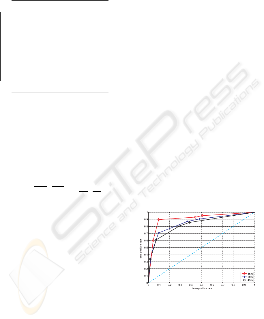
Table 1: Iterative search algorithm.

1. compute candidates φ

, j = (1, .., m) for

which P

(Y|φ

) > T

2. initialise φ

, j ∈ (1, .., m) for object part i = 1;

set k = i; for each candidate φ

...

(a) ...vote for reference point φ

based on part

location φ

(b) ...set i = i+ 1 and k = [k;i]

from φ

and compute

(Φ

∗

|Y), with Φ

∗

= (φ

)

(d) ...IF P

(Φ

∗

|Y) > T: go back to (a);

...ELSE: end

also on a global scale, expressing the relationships be-

tween labels and global image features. In this work

this is the predicted distribution of object categories

in the image which helps to achieve globally con-

sistent recognition. Based on the work presented in

(Bachmann and Balthasar, 2008) we exploit the re-

lation between the expected distribution of a certain

category and the scenery. The scene-based informa-

tion is formally introduced into our framework by ex-

tending Equation (5) with a context-awareobject prior

predicting the distribution of category labels

Ψ(E, l, θ) = Ψ(E, l, v, ξ,Φ)

| {z }

local information

∑

i=1

|Y)

| {z }

context information

(19)

with category context potential

|Y) = logP(l

) . (20)

(·) predicts the label l

from a global perspective

using global image features M

. The global features

characterise the entire image in terms of magnitude

and orientation of edges in different image resolu-

tions. For this work we deﬁned a set of scene cate-

gories c

= {

open, semi-open, closed

}, each ex-

pressed by a unique feature vector M

, describing the

openness of the scene. This information is used to de-

rive the distribution of category labels and category

probability in the image. The feature vector M

for

each speciﬁc scene has been calculated from a train-

ing data set and is formally expressed by a mixture of

Gaussian model. The relationships between the con-

textual features and a speciﬁc object category c

has

been learned in a training stage as presented in (Bach-

mann and Balthasar, 2008). Given an input image, the

prior probability of an object category c

is expressed

as its marginal distribution over all scene categories c

whereas the scene similarity of the input image (ex-

pressed by M

obs

) to the deﬁned scene categories is

determined by calculating the joint probability with

the single components in M

3 EXPERIMENTAL RESULTS

This section presents the experimental evaluation of

the object detection approach developed in the pre-

vious sections. The results are based on image se-

quences of typical urban trafﬁc scenarios. The al-

gorithm is initialised automatically by scanning for

the actual number of dominant motions in the scene.

Concerning the motion of the observer, the road plane

is determined at the beginning of the image sequence

as described in (Duchow et al., 2006). Thus, the mo-

tion proﬁle of the observer can be determined by sam-

pling feature points exclusively from the region that

is labeled as road plane and therefore static relative

to the observer. During the segmentation process, the

motion proﬁles are reﬁned and updated continuously

with the motion tracker scheme described in (Bach-

mann and Dang, 2008). Regarding the relative im-

portance of data and smoothness term in the segmen-

tation process, the regularization factor was adapted

empirically to values between λ = (0.05, .., 0.5).

The conﬁdence of an image point to be part of

an object hypothesis, i.e. label, is calculated based

on its relative motion, its position and similarity to

the deﬁned object categories. The image point is as-

signed to the label with highest conﬁdence. The train-

ing data for object category

car

as presented here was

extracted from an image data base of 160 images.

Figure 3: ROC-curve for rear view of object category

car

as a function of the distance from the observer.

Figure 3 shows that a threshold value of T ≈ 0.6

yields a good compromise between a reasonable true

positive rate and a false positive rate at relative low

values.

Figure 4 shows some of the detection results for

object category

car

. The model was learned from

VISAPP 2009 - International Conference on Computer Vision Theory and Applications

296

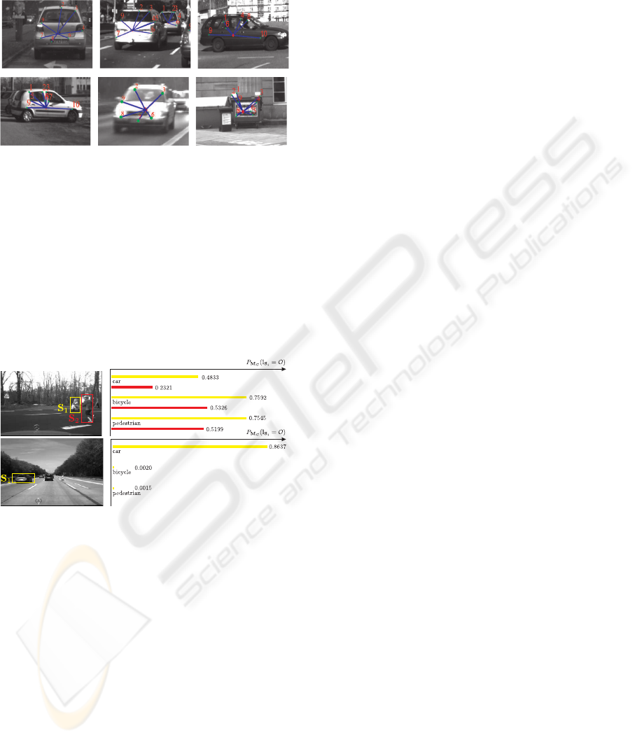
labeled data. The patch-size of the extracted inter-

est points was scale-normalised based on a predeﬁned

reference scale.

Figure 4: Detection results (threshold value T = 0.5) for

object category

car

. The ﬁgure on the bottom right shows

a false positive.

Figure 5 shows the classiﬁcation results for de-

tected objects solely based on scene context. No lo-

cal category information has been integrated. It can

be seen that the integration of global information is

useful as a ﬁrst process of image recognition. Joint

use of the proposed local object detector together with

category-speciﬁc scene context improves the recogni-

tion accuracy as shown in Figure 6.

Figure 5: Left: Detected objects based on the local ob-

ject properties motion similarity and position. Right: Prior

probability P

= O) of image region S

to belong to ob-

ject category O = {

car, bicycle, pedestrian

} solely

based on scene context information.

Here, the object detection and segmentation re-

sults for different trafﬁc scenes is depicted. As in this

work only object category

car

is known locally to the

system, detected objects that are labeled

bicyclist

pedestrian

rely solely on the global context of the

image. In the initialization phase of the segmentation

process the motion estimates for the labels are inac-

curate. Therefore the segmentation is mainly driven

by the appearance-based conﬁdence measure. With

increasing accuracy and distinctiveness of the labels

motion proﬁle, the inﬂuence of the motion cue in-

creases. In most cases, it takes less than 3 frames to

partition the image into meaningful regions.

4 CONCLUSIONS

This paper has presented a MRF for pixel-accurate

object recognition that models local object informa-

tion and global information explicitly. The local in-

formation consists of a set of distinct 6-dof motion

proﬁles, positions and - on a high abstraction level

- the local appearance similarity to the trained ob-

ject category

car

. Distinctive, local object descriptors

and a structural prior on the object-parts conﬁguration

have been extracted from a set of sample images. The

structural relationships among object parts has been

modelled as sparse structural prior. Object recogni-

tion is realised by an iterative method that ﬁnds an

optimal conﬁguration of the object parts based on the

local appearance in the image and its spatial arrange-

ment. Global information is derived from scene-based

information generated according to the scene of the

input image. As the occurrence of object categories is

closely related to the scene of the image, scene con-

text is exploited to derive characteristic category dis-

tributions and probabilities. It has been shown that

the joint use of a local object detector and scene con-

text improves the recognition accuracy. Under the as-

sumption of motion and category homogeneity within

the boundaries of an object, spatial consistency has

been modelled through a Markov Random Field.

In ongoing work, we expect to increase the perfor-

mance of the method by further reﬁning and extend-

ing the sparse object model description. We suppose

to increase the quality of the classiﬁcation process by

making the object appearance descriptors invariant to

object orientation and rotation. Additionally, the per-

formance shall be increased by an exhausting train-

ing of different object categories. Furthermore it is

intended to speed up the search algorithm that incor-

porates the object spatial conﬁguration to make the

entire process computationally feasible.

ACKNOWLEDGEMENTS

This work was partly supported by the Deutsche

Forschungsgemeinschaft DFG within the collabora-

tive research center ‘Cognitive Automobiles’.

REFERENCES

Bachmann, A. and Balthasar, M. (2008). Context-aware ob-

ject priors. In IEEE IROS 2008; Workshop on Plan-

ning, Perception and Navigation for Intelligent Vehi-

cles (PPNIV), Nice, France.

BAYESIAN SCENE SEGMENTATION INCORPORATING MOTION CONSTRAINTS AND CATEGORY-SPECIFIC

INFORMATION

297

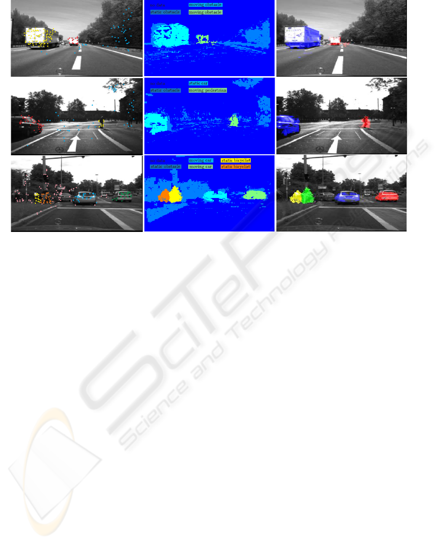
Figure 6: Left: Scenes with a variable number of moving objects. The 6–dof motion for each object is determined based

on a set of interest points extracted from the respective object. Coloured markers indicate the tracked points. Middle: The

resulting segmentation map. Each image point is assigned the label containing the most probable motion proﬁle and position.

Right: The segmented image. Image points assigned to an object label are highlighted.

Bachmann, A. and Dang, T. (2008). Improving motion-

based object detection by incorporating object-

speciﬁc knowledge. International Journal of Intel-

ligent Information and Database Systems (IJIIDS),

2(2):258–276.

Besag, J. (1974). Spatial interaction and the statistical anal-

ysis of lattice systems. Journal of the Royal Statistical

Society, Series B 36(2):192–236.

Burl, M. C., Weber, M., and Perona, P. (1998). A probabilis-

tic approach to object recognition using local photom-

etry and global geometry. Lecture Notes in Computer

Science, 1407:628ff.

Crandall, D. and Huttenlocher, D. (2007). Composite mod-

els of objects and scenes for category recognition. In

Proc. IEEE Conference on Computer Vision and Pat-

tern Recognition CVPR ’07, pages 1–8.

Dang, T., Hoffmann, C., and Stiller, C. (2006). Self-

calibration for active automotive stereo vision. In Pro-

ceedings of the IEEE Intelligent Vehicles Symposium,

Tokyo.

Duchow, C., Hummel, B., Bachmann, A., Yang, Z., and

Stiller, C. (2006). Akquisition, Repraesentation und

Nutzung von Wissen in der Fahrerassistenz. In In-

formationsfusion in der Mess- und Regelungstechnik

2006, VDI/VDE-GMA. Eisenach, Germany.

Fischler, M. and Elschlager, R. (1973). The representa-

tion and matching of pictorial structures. IEEE Trans.

Comput., 22(1):67–92.

Geman, S. and Geman, D. (1984). Stochstic relaxation,

Gibbs distribution, and the Bayesian restoration of im-

ages. In IEEE Transaction on Pattern Analysis and

Machine Intelligence, volume 6, pages 721–741.

Harris, C. and Stephens, M. (1988). A combined corner

and edge detector. In Fourth Alvey Vision Conference,

Manchester, pages 147–151.

He, X. and Yung, N. (2004). Curvature scale space corner

detector with adaptive threshold and dynamic region

of support. In 17th International Conference on Pat-

tern Recognition, volume 2, pages 791–794, Washing-

ton, DC, USA. IEEE Computer Society.

Ohm, J.-R. and Ma, P. (1997). Feature-Based cluster seg-

mentation of image sequences. In ICIP ’97-Volume 3,

pages 178–181, Washington, DC, USA. IEEE Com-

puter Society.

Rentschler, I., Juettner, M., Osmana, E., Mueller, A., and

Caell, T. (2004). Development of conﬁgural 3D object

recognition. Elsevier - Behavioural Brain Research,

149(149):107–111.

Rockwell, T. (1972). Skills, judgment, and information ac-

quisition in driving. Human Factors in Highway Traf-

ﬁc Safety Research, pages 133–164.

Sivak, M. (1996). The information that drivers use: is it

indeed 90% visual? Perception, 25(9):1081–1089.

VISAPP 2009 - International Conference on Computer Vision Theory and Applications

298