
TRANSFORM CODING OF RGB-HISTOGRAMS
Reiner Lenz
Dept. Science and Engineering, Link
¨
oping University, SE-60174 Norrkping, Sweden
Pedro Latorre Carmona
Departamento de Lenguajes y Sistemas Informaticos, Universidad Jaume I, 12071 Castellon de la Plana, Spain
Keywords:
RGB-Histograms, Image Databases, Finite Groups, Harmonic Analysis.
Abstract:
In this paper we introduce the representation theory of the symmetric group S(3) as a tool to investigate the
structure of the space of RGB-histograms. We show that the theory reveals that typical histogram spaces are
highly structured and that these structures originate partly in group theoretically defined symmetries. The
algorithms exploit this structure and constructs a PCA like decomposition without the need to construct cor-
relation or covariance matrices and their eigenvectors. We implemented these algorithms and investigate their
properties with the help of two real-world databases (one from an image provider and one from a image search
engine company) containing over one million images.
1 INTRODUCTION
The number and size of image collections is growing
steadily and with it the need to organize, search or
browse these collections. These collections can also
be used to study the statistical properties of large col-
lections of visual data and to derive models of their
internal structure.
In this paper we are interested in the understand-
ing of the statistical structure of large image collec-
tions and in the design of algorithms for applications
where huge numbers of images have to be processed
very fast. Therefore our motivation lies in methods
that are applicable to huge databases and enable fast
response times.
We will investigate the color properties of images
using one of the simplest and fastest color descrip-
tors available: the RGB histogram (Swain and Bal-
lard, 1991; Hafner et al., 1995). We will analyze the
structure of the space of RGB histograms and algo-
rithms for their fast processing and structure reduc-
tion.
The approach we use is based on the observation
that compression and fast-processing methods are of-
ten tightly related to the underlying structure of the in-
put signal space. This structure can often be described
in terms of transformation groups. The best-known
class of algorithms of this type are the FFT-methods
based on the group of shift operations. In the sig-
nal processing field these methods were generalized
to the application of finite groups with applications to
filtering, and pattern matching and computer vision.
See (Cooley and Tukey, 1965; Holmes, 1979; Lenz,
1994; Lenz, 1995; Lenz, 2007; Rockmore, 2004) for
some examples.
3D (like RGB) Histograms have a wide variety of
applications in image processing, ranging from image
indexing and retrieval (Sridhar et al., 2002; Yoo et al.,
2002; Geusebroek, 2006; Smeulders et al., 2000) to
object tracking (Comaniciu et al., 2003) to cite a few.
In the following we will first argue that a rele-
vant transformation group for the space of RGB his-
tograms is the group S(3) of permutations of three
objects. We will describe the basic facts from the rep-
resentation theory of S (3) and investigate the proper-
ties of the resulting transforms of histograms. As a
result we will see that the generated structures have a
PCA like decorrelation property.
We will apply these transforms to very large col-
lections of images. One consisting of 760000 images
representing the collection of an image provider and
one with 360000 images from the database of an im-
age search engine.
117
Lenz R. and Latorre Carmona P. (2009).
TRANSFORM CODING OF RGB-HISTOGRAMS.
In Proceedings of the Fourth International Conference on Computer Vision Theory and Applications, pages 117-124
DOI: 10.5220/0001653501170124
Copyright
c
SciTePress

2 NOTATIONS AND BASIC FACTS
We first summarize a few facts about permutations
and representation theory and then we will describe
how to generalize this to representations on spaces of
RGB histograms. We only mention the basic facts and
the interested reader should consult one of the books
in the field, for example (Serre, 1977; Diaconis, 1988;
Fulton and Harris, 1991; F
¨
assler and Stiefel, 1992;
Chirikjian and Kyatkin, 2000).
The permutations of three objects form the sym-
metric group S(3). This abstract group comes in
several realizations and we will freely change be-
tween them. In the most abstract context the per-
mutations π are just elements of π ∈ S(3). We will
use it to investigate color images. We describe col-
ors in the RGB coordinate system described by triples
(R,G,B). If we want to denote a triple with some
numerical values then we write (aaa),(aab), (abc) in
the cases where all three, two or none of the val-
ues are equal. If a permutation changes the order
within the triple we will simply use the new order of
the generic RGB triple as a symbol for the permu-
tation. The permutation (RBG) leaves the first ele-
ment fixed and interchanges the other two. It should
be clear from the context if we mean RGB-triples
like (abc) or permutations like (RBG). We define
the special permutations π
c
as the cyclic shift π
c
=
(BRG) and π
r
as the reflection (RBG). These two
permutations are the generators of S (3) and all oth-
ers can be written as compositions of these two. The
group S (3) has six elements and we usually order
them as π
0
c
,π
c
,π
2
c
,π
r
,π
c
π
r
,π
2
c
π
r
or in RGB notation
(RGB),(BRG),(GBR),(RBG), (GRB),(BGR)
We see that the three even permutations π
0
c
,π
c
,π
2
c
form a commutative subgroup with the same proper-
ties as the group of 0, 120, 240 degrees rotations in the
plane. The remaining odd permutations are obtained
by preceding the even permutation with π
r
.
If we consider the triples (R,G,B)
0
as vectors x
in a three-dimensional vector space then we see that
we can describe the effect of the permutations by a
linear transformation described by a matrix. In this
way the permutations π
c
,π
r
are associated with the
matrices T
G
(π)
T
G
(π
c
) =
0 0 1
1 0 0
0 1 0
T
G
(π
r
) =
1 0 0
0 0 1
0 1 0
(1)
This is the simplest example of a representation
of S (3) which is a mapping from the group to ma-
trices so that group operations go over to matrix mul-
tiplications. In this case the matrices are of size 3 ×3
3 Orbit (255 0 0)
6 Orbit (255 128 0)
Figure 1: Examples of a three- and a six-orbit.
and we say that we have a three-dimensional rep-
resentation. The elements π
c
,π
r
generate S(3) and
therefore we find that also all six permutation matri-
ces are products of T
G
(π
c
),T
G
(π
r
).
If we apply all six permutations to triples (abc)
we obtain the so called orbits. For triples with differ-
ent values for a, b and c we generate six triples, if we
apply them to a triple (abb) we get three triples and
the triple (aaa) is invariant under all elements in S (3).
The orbits of S(3) have therefore length six, three and
one respectively. We denote a general orbit by O and
the orbits of length one, three and six by O
1
,O
3
,O
6
.
Two such orbits are illustrated in Fig.1 where each
stripe shows one element in the orbit. For the three-
orbit the colors are repeated for the odd permutations
since the last two values in the RGB triple for the red
image are identical.
We can use the concept of an orbit to construct
new representations similar to those in Eq. (1). Take
the six-orbit O
6
. We describe each element on O
6
by
one of the six unit vectors in a six-dimensional vector
space. Since permutations map elements in the orbit
to other elements in the orbit we see that each permu-
tation π defines a 6 ×6 permutation matrix T
6
(π) in
the same way as those in Eq. (1). Also here it is suf-
ficient to construct T
6
(π
c
) and T
6
(π
r
). The same con-
struction holds for the three-orbits O
3
. For the one-
orbit the matrices are simply the constants T
1
(π) = 1.
We denote these vector spaces (defined by the orbits)
by V
1
,V
3
,V
6
.
The row- and column sums of permutation matri-
ces are one and we see that T (π)1 = 1 where T (π) is
a permutation matrix and 1 =
1 ... 1
is a vec-
tor of suitable length with only elements equal to one.
This shows that the subspaces V
t
k
of V
k
,(k = 1,3, 6),
spanned by 1 are invariant under all operations with
permutation matrices. These spaces define the triv-
ial representation of S (3) (Fulton and Harris, 1991;
F
¨
assler and Stiefel, 1992).
Since V
t
k
is an invariant subspace of V
k
,(k =
1,3,6) we see that their orthogonal complements are
also invariant and we have thus decomposed the in-
variant spaces V
k
into smaller invariant spaces and
each of these subspaces defines a lower-dimensional
representation (smaller matrices) of the group. The
smallest such invariant spaces define the irreducible
representations of the group (for definitions and ex-
amples see (Serre, 1977; Fulton and Harris, 1991;
VISAPP 2009 - International Conference on Computer Vision Theory and Applications
118

F
¨
assler and Stiefel, 1992)).
The decomposition for the three-dimensional
space V
3
is given by the matrix
P
3
=
1
√
3
1 1 1
√
2
√
2cos(2π/3)
√
2cos(4π/3)
0
√
2sin(2π/3)
√
2sin(4π/3)
=
e
1
P
2
(2)
where we identify the basis vector for the sub-
spaces V
t
3
in the first row. The orthogonal comple-
ment is spanned by the remaining two basis vectors
and it can be shown that the space V
s
3
spanned by these
two cannot be split further. This defines another irre-
ducible representation, known as the standard repre-
sentation see (Fulton and Harris, 1991).
For the six-dimensional space V
6
it can be shown
that the decomposition into irreducible representa-
tions is given by
P
6
=
b
1
b
1
b
1 −
b
1
P
2
0
0 P
2
(3)
where
b
1 represents 3D vectors with entries
1
√
6
and P
2
is the matrix with the two basis vectors defined in
Eq.(2).
In the final stage of the construction we describe
how the group operates on RGB histograms. We
start with an orbit O with elements o. The permu-
tations π are maps π : O →O. Now take a linear func-
tion f : O → R; o 7→ f (o). We then define the new
function f
π
by f
π
(o) = f (π
−1
(o)). It can be shown
that this defines a representation of S(3) on the space
of functions on the orbit. These representations can
be reduced in the same manner as we did with the
representations on the orbit.
For our application the functions of interest are
the histograms. We will however modify this idea
slightly. We consider a simple example first. Select
an orbit O with elements o and assume that we have
a probability distribution on O. Since O has finitely
many elements this is a histogram h with the prop-
erties that h(o) ≥ 0 and
∑
o∈O
h(o) = 1. Applying a
permutation π to the orbit elements defines a new his-
togram h
π
. In the usual framework of representation
theory we have orthonormal matrices T (π) transform-
ing vectors according to h 7→ T (π)h. We thus have
two transformations h 7→ h
π
and h 7→ T (π)h. The
first of this preserves the L
1
-norm while the other pre-
serves the L
2
-norm. We avoid this conflict and con-
sider the square-roots of the probabilities instead (see
also (Srivastava et al., 2007)). In the following we use
the definition:
h(o) =
p
p(o) (4)
where p(o) is the probability of the orbit element o
and h(o) is the modified ”histogram”.
We summarize the construction so far as follows:
• Split the RGB space into subsets X such that the
split is compatible with the permutations in S (3).
We call the elements of these subsets bins and de-
note them by x.
• For a set of images compute the probabili-
ties p(x),x ∈X
• Convert and collect them in histogram vectors h
with entries h(x) =
p
p(x).
• Collect bins x that are related by permutations in
orbits O
i
. This defines a partition X =
S
i
O
i
• Every orbit O defines a representation of dimen-
sion one, three or six
• Split three-dimensional representations into two
parts using the matrix P
3
defined in Eq.(2)
• Split six-dimensional representations into four
parts using the matrix P
6
defined in Eq.(3)
• Leave the one-dimensional representations as they
are
• The final decomposition is now:
V = V
t
⊕V
a
⊕V
s
(5)
where V is the space defined by the bins. The
space V
t
is the invariant subspace associated with
the one-point orbits and the invariant parts (first
rows in P
3
,P
6
) of the three and six point orbits. V
a
is the subspace associated with the six-point orbits
and depends on the even/odd properties (second
row in P
6
) of the six point orbits. The V
s
part fol-
lows the P
2
parts in the three- and six-point orbit
transforms, Eqs.(2, 3).
3 IMPLEMENTATION
In the derivation we only required that the split of the
RGB space is compatible with the operation of S(3).
Since we are interested in fast implementations we
will only consider very regular partitions where we
split the R, G and B intervals into eight bins each,
leading to a 512D RGB histogram. The procedure
is easily generalized to all equal partitions of the
axis into β bins leading to β
3
dimensional RGB his-
tograms. Due to the exponential growth, values β ≤8
are most realistic.
TRANSFORM CODING OF RGB-HISTOGRAMS
119
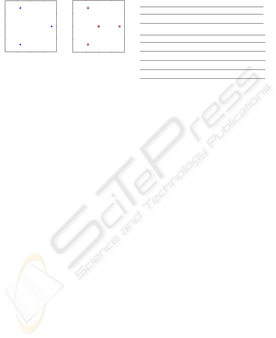
−1 −0.5 0 0.5 1
−1
−0.5
0
0.5
1
1
4
2
5
3
6
3 Orbit (255 0 0)
−1 −0.5 0 0.5 1
−1
−0.5
0
0.5
1
6−Orbit (255, 128,0)
Figure 2: Orbit decompositions for the standard representa-
tion block.
For eight bins per channel we use octal representa-
tions of the bin-number and write (klm) for the num-
ber k + 8l + 64m. One-point orbits are invariant un-
der all permutations, therefore they represent gray-
values (kkk). Black is characterized by (000) and
white by (777). The three-orbits are given by bin
numbers (kll). Consider as example the images given
by the stripes in the left part of Fig. 1. The histogram
for the first stripe has a one at position (700). Ap-
plying the six permutations we get the six stripes in
this figure and six histograms. Applying the transfor-
mation P
3
to the three-orbit section of the histogram
space given by (700),(070),(007) we find that the
first entry is always one and the positions in the other
two dimensions (the P
2
part) transform as in an equal
sided triangle as shown in the left part of Figure 2.
These two-dimensional vectors transform thus as 120
degrees rotations under permutations.
The orbit of (740), representing the RGB vector
(255,128,0), are the six stripes in the right part of Fig-
ure 1. Using the decomposition defined by P
6
we get
two two-dimensional vectors (from the last four rows
of the matrix). We see the projection of the six or-
bit colors to these subspaces in the right part of Fig-
ure 2. The points marked with an ”o” belong to one
subspace, the ”+” points to the other.
The coordinates of the projections into the alter-
nating and the standard parts are collected in Table 1
We have now described how to reorganize the his-
tograms so that the different components show sim-
ple transformation properties under channel permuta-
tions. This is one of the advantages of this approach.
The other is the relation to principal component anal-
ysis (PCA) that we will explain now.
We start with a simple example. Consider a vec-
tor h defined on an three-point orbit. Generate all
different versions h
π
under permutations and com-
pute the matrix C =
∑
π
h
π
h
π
0
. It is invariant under
a re-ordering of the orbit since this will simply re-
arrange the sum. This is the simplest example of
an S (3)-symmetric matrix. We generalize this to the
Table 1: Coordinates of projections for six-point orbits.
Alternating Representation
RGB GBR BRG RBG GRB BGR
0.408 0.408 0.408 -0.408 -0.408 -0.408
Standard Representation
RGB GBR BRG RBG GRB BGR
0.817 -0.408 -0.408 0 0 0
0 -0.707 0.707 0 0 0
0 0 0 -0.408 0.817 -0.408
0 0 0 0.707 0 -0.707
definition of a wide-sense-stationary process as fol-
lows: Assume that we have vectors h in a vector
space V and the permutations π ∈ S (3) operate on
these vectors by h 7→ h
π
. Assume further that we
have a stochastic process with stochastic variable ω
and values in h
ω
∈V . We define the correlation ma-
trix Σ of this process as Σ = E
h
ω
h
ω
0
where E(.)
denotes the expectation with respect to the stochastic
variable ω. Assume further that we have a representa-
tion T (π) on V .
Definition. The stochastic process with correlation
matrix Σ is T -wide-sense stationary if T (π)Σ = ΣT (π)
for all π ∈ S (3).
We will only consider representations for which
the matrices T are orthonormal and in this case
we have Σ = T (π)ΣT (π)
0
for all π ∈ S (3).
But T (π)ΣT (π)
0
is the correlation matrix of the
stochastic process h in the new coordinate sys-
tem T(π)h and we see that wide-sense-stationarity
means that the correlation matrix is independent of
a certain class of coordinate transforms.
The general theory (Schur’s Lemma, (F
¨
assler and
Stiefel, 1992)) shows that we can find a matrix U
(defining a new basis in the vector space) such that
the correlation matrix in the new space is block diag-
onal. This matrix U depends only on the group S (3) :
Theorem 3.1. For an S(3)-symmetric process with
correlation matrix Σ we can find a matrix U such that:
UΣU
0
=
Σ
t
0 0
0 Σ
a
0
0 0 Σ
s
(6)
This transformation h 7→Uh defines a partial principal
component analysis of the histogram space by block-
diagonalizing the correlation matrix and it is given by
the construction described in the previous Section 2.
VISAPP 2009 - International Conference on Computer Vision Theory and Applications
120
4 EXPERIMENTS
We implemented the transform described above and
used it to investigate the internal structure of two
large image databases. One of the image databases
(we denote it by PDB) contains images from an im-
age provider. It consists of 754034 (watermarked)
images and is used on their website. The second
database (referred to as SDB) contains 322903 im-
ages collected from the internet by a commercial im-
age search engine. They are indexed by 31 differ-
ent keyword categories ranging very general concepts
like “beach” to very special like “Claude Monet”.
In all experiments we computed first the RGB his-
tograms p for all these image and then the square-
root of the histogram entries. In all experiments we
used eight bins/channel. We get 8 one-point orbits,
56 three-point orbits and 56 six-point orbits. The di-
mensions of the blocks described in Eq.(6) are there-
fore (120,56, 336). We apply the transform resulting
in the new vector v = (v
t
,v
a
,v
s
) corresponding to the
vector spaces in Eq.(5).
We describe first some of our experiments regard-
ing the statistical properties of these databases and
then we illustrate the compression properties of the
group theoretical transform in Section 3.
We first computed the norms of the vectors v
t
,v
a
and v
s
, their mean and max value of
k
v
a
k
2
for PDB
and SDB. The coefficients in v
a
(see also Table 1) are
given by differences between contributions from even
permutations and odd permutations in a six-orbit. If
we assume that even and odd permutations are statis-
tically equally likely then we expect the value of these
coefficients to be small on average. We also computed
the histogram (with 1000 bins) of these norms
k
v
a
k
2
and computed the ratio between the probability of the
first bin (with the small values of the norm) and the
sum over the remaining bins (representing the non-
zero norm values). The results are collected in Ta-
ble 2.
Table 2: Contributions of the coefficients.
Database E
k
v
t
k
2
E
k
v
a
k
2
E
k
v
s
k
2
Max(
k
v
a
k
2
) zero vs. non-zero
PDB 0.606 0.042 0.350 0.312 0.057
SDB 0.678 0.031 0.291 0.278 0.144
This shows that the main contribution comes
form v
t
and the contributions from v
a
are indeed low.
We also see that there is a difference between the two
databases where the contribution of the v
a
is higher
for PDB. One reason for this could be the higher pro-
portion of cartoon-like images with distinct color dis-
tributions in PDB as compared with SDB.
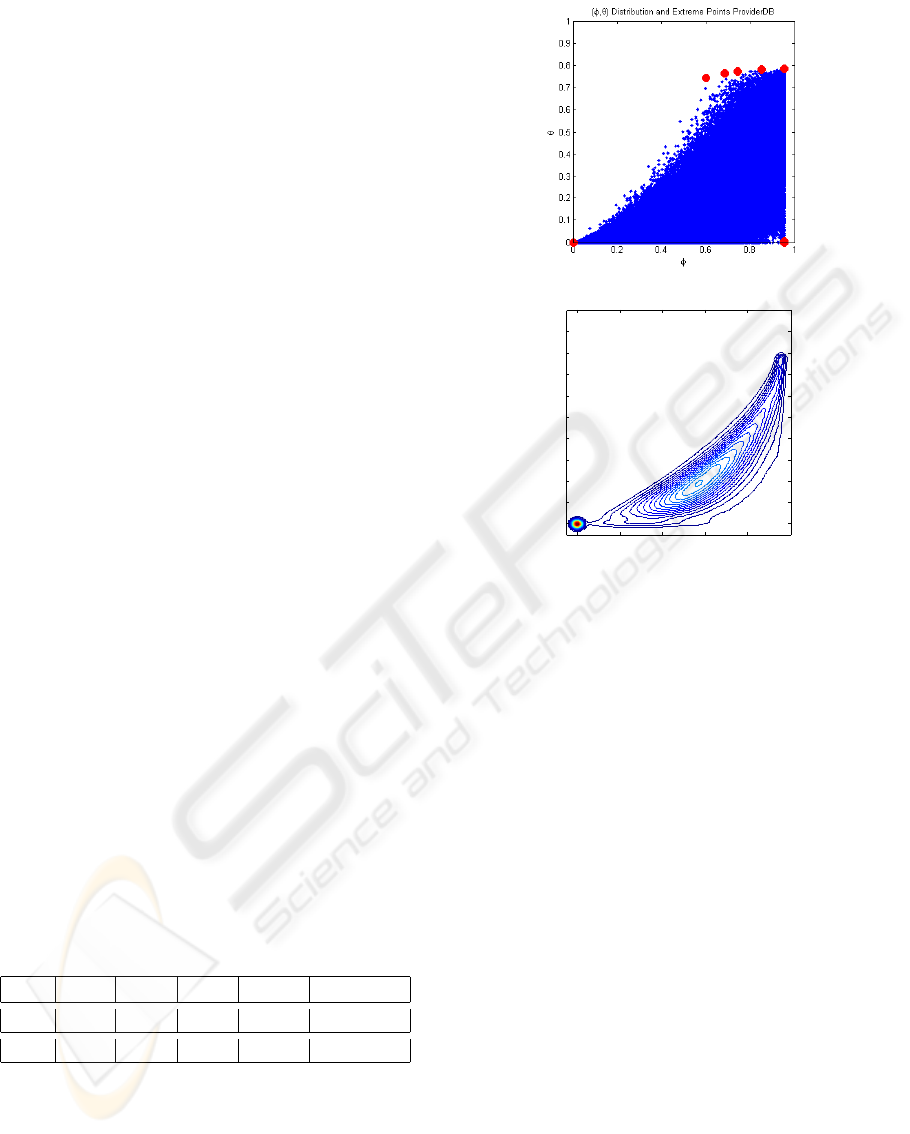
φ
θ
Probability Density for Provider DB
0 0.2 0.4 0.6 0.8 1
0
0.1
0.2
0.3
0.4
0.5
0.6
0.7
0.8
0.9
1
Figure 3: Location and probability distribution from PDB.
From the construction we know that the mod-
ified histograms and their transforms are unit vec-
tors
k
v
k
2
=
k
v
t
k
2
+
k
v
a
k
2
+
k
v
s
k
2
= 1. Since
k
v
a
k
2
is small we conclude that the 3D v = (v
t
,v
a
,v
s
) are
concentrated in the neighborhood of one quarter of a
great circle of the unit sphere. The length of v
t
is also
larger than the length of v
s
. Based on these heuristic
considerations we introduce the following polar coor-
dinate system on the unit vectors given by the norms
of the projection vectors:
v
t
,v
a
,v
s
= (cos ϕcosθ,cos ϕsin θ,sinϕ) (7)
The angle ϕ corresponds to the latitude and we
think of it as an indication of the unbalance between
the three channels (for a value of zero all the con-
tribution is in the v
t
part). The (longitudal) angle θ
is a measure of the contribution of v
a
. The (ϕ,θ)-
distribution of the images (every dot corresponds to
one image) in the PDB is shown in the upper plot
of Figure 3. The corresponding probability density
distribution is shown in the lower plot. This figure
shows that the distribution of the images is concen-
trated around the origin and that the distribution has a
banana-like shape in the (ϕ,θ)-space.
The positions of the eight extreme points of the con-
vex hull are marked with filled circles in the upper
TRANSFORM CODING OF RGB-HISTOGRAMS
121
(0,0)
(0.85,0.78)
(0.95,0)
(0.74,0.77)
(0.96,0.0042)
(0.69,0.77)
(0.96,0.79)
(0.6,0.75)
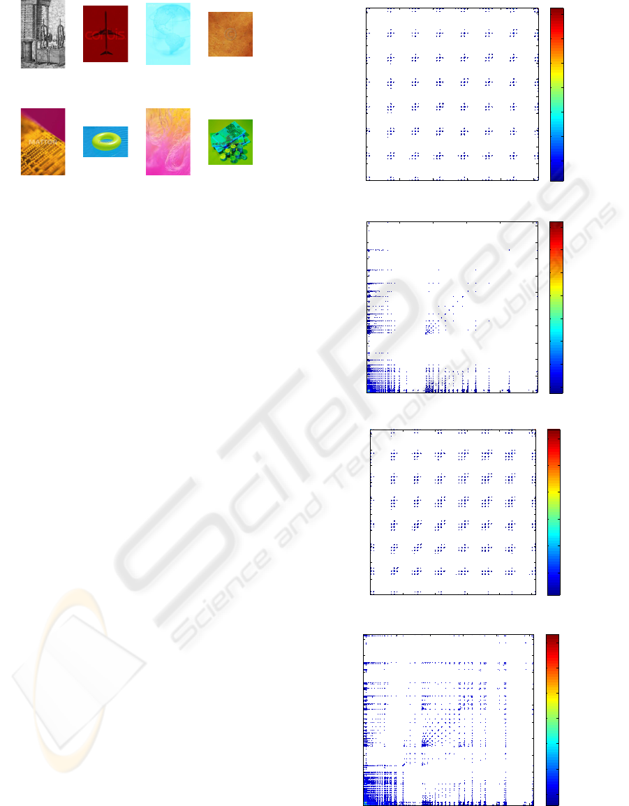
Figure 4: Extreme images in PDB.
plot of Figure 3. The images belonging to the eight
extreme points of the convex hull are shown in Fig-
ure 4.
Theorem 3.1 shows that wide-sense-stationary
processes are partially decorrelated by the transform.
In the remaining part of this section we will now
investigate if the two databases define wide-sense-
stationary processes.
We illustrate the effect of the transform on the
correlation matrix in Figure 5 showing the contour
plots of the correlation matrices computed from the
square-root transformed histograms before and after
the transformation. It can be clearly seen that the ef-
fect of the transformation is a concentration in the first
120 components given by the vectors v
t
.
In the following experiment we evaluated the ap-
proximation error introduced by reducing the cor-
relation matrix computed from the transformed his-
tograms (Figure 5) to the block-diagonal matrix with
block-sizes (120,56, 336). We computed the first 20
eigenvectors of the full correlation matrices and found
that they explain about 85% of the summed eigen-
values for both databases. We also computed the
20 eigenvectors for the block-structured correlation
matrix. From the construction of the blocks we ex-
pect that these eigenvectors of the block-diagonal ma-
trix are elements of the 120, 56 or 336-dimensional
subspaces defined by the blocks. In Table 3 we il-
lustrate the accumulated, normed eigenvalues A
K
=
(
∑
γ
K
k=1
)/(
∑
γ
512
k=1
) where γ
k
is the k-th eigenvalue and
to which block the different eigenvectors belong. We
see the minor role of the coefficients in v
a
: the only
eigenvectors from the second block are in positions
nine and eleven (last one not shown in Table 3).
Also here we see that PDB has a higher contribution
from v
a
.
To get a more quantitative measure on how good
the block-diagonal eigenvalues approximate the full
Correlation Matrix Search DB
100 200 300 400 500
50
100
150
200
250
300
350
400
450
500
0.02
0.04
0.06
0.08
0.1
0.12
0.14
Transformed Correlation Matrix Search DB
100 200 300 400 500
50
100
150
200
250
300
350
400
450
500
0
0.02
0.04
0.06
0.08
0.1
0.12
0.14
Correlation Matrix Provider DB
100 200 300 400 500
50
100
150
200
250
300
350
400
450
500
0.02
0.04
0.06
0.08
0.1
0.12
Transformed Correlation Matrix Provider DB
100 200 300 400 500
50
100
150
200
250
300
350
400
450
500
0
0.02
0.04
0.06
0.08
0.1
0.12
Figure 5: Original and transformed correlation matrices.
VISAPP 2009 - International Conference on Computer Vision Theory and Applications
122
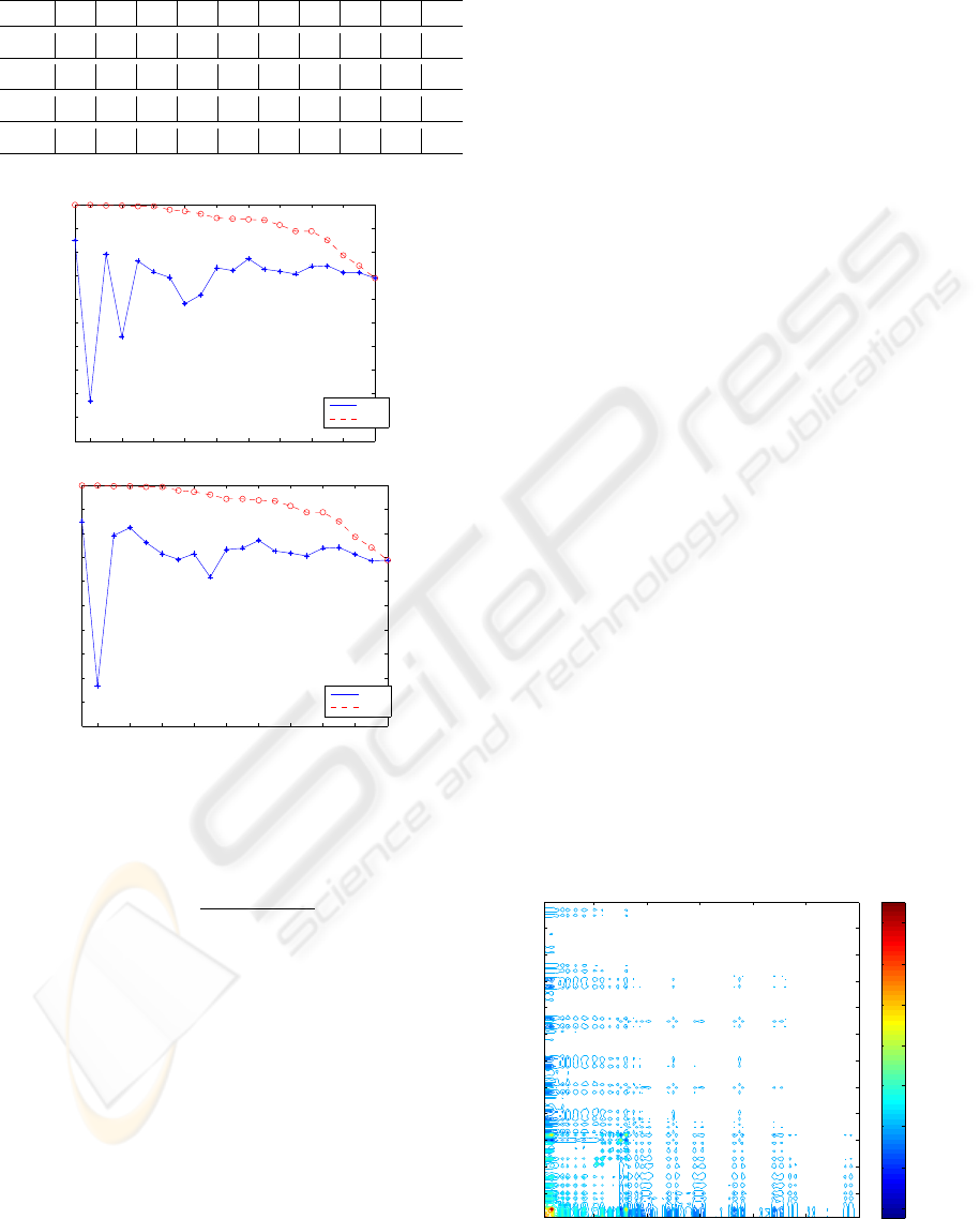
Table 3: Accumulated Eigenvalues and Block-Number for
the Block-Diagonal Eigenvectors.
1 2 3 4 5 6 7 8 9 10
SDB 0.40 0.51 0.57 0.62 0.65 0.67 0.70 0.72 0.74 0.75
Block 1 1 3 1 1 3 1 3 3 3
PDB 0.41 0.49 0.55 0.59 0.63 0.66 0.68 0.70 0.71 0.72
Block 1 3 1 1 3 1 3 3 2 1
2 4 6 8 10 12 14 16 18 20
0.5
0.55
0.6
0.65
0.7
0.75
0.8
0.85
0.9
0.95
1
Search DB
γ(mm)
γ(20n)
2 4 6 8 10 12 14 16 18 20
0.5
0.55
0.6
0.65
0.7
0.75
0.8
0.85
0.9
0.95
1
Provider DB
γ(mm)
γ(20n)
Figure 6: Projection properties of the approximation.
matrix eigenvectors we computed the approximation
values:
γ
m,n
=
∑
n
k=1
e
B
m
b
k
n
(8)
where
e
B
m
is the matrix of the m first eigenvectors of
the block-diagonal approximation and b
k
is the k-th
eigenvector of the full correlation matrix. The value
of γ
m,n
is a normalized measure on how large part of
the n first eigenvectors of the full correlation matrix
are projected into the space of the first m eigenvec-
tors of the block-diagonal matrix. Some of the re-
sults are shown in Figure 6 where the solid line shows
the values of γ
mm
,m = 1..20 (equal number of full
and block-diagonal eigenvectors) and the dashed line
shows γ
20,n
, the result for the full set of 20 eigenvec-
tors of the block-diagonal matrix.
We see that the first 20 eigenvectors explain about
85% of the contributions from the first 20 eigenvec-
tors of the full correlation matrix. Since the contri-
bution from the last eigenvectors to the total variation
(see also Table 3) is small we find that the approxi-
mation computed from the block-diagonal matrix is
probably sufficient for most applications.
5 EXTENSIONS
AND CONCLUSIONS
The experiments described so far show that the trans-
form, derived from the assumption that permutations
of the R, G and B channels are likely to occur with
the same probabilities, lead to a separation of the
histogram space into three clearly separated blocks.
From an S(3) point of view nothing can be said about
the internal structure of these blocks and if we want
to transform them we have to use different sources of
information about them. In the previous section we
used standard PCA to identify important sections of
these parts of the space. We also implemented a sec-
ond transform that takes into account the multilevel
structure given by the different bin sizes. All experi-
ments described so far used an eight-bin quantization
of the RGB axis resulting in a 512D RGB histogram.
If we reduce the number of bins by a factor of 2 we
get 4
3
= 64 bin RGB histograms and at the next level
we have only 2 ×2 ×2 = 8 bins left. Bin reduction
and channel permutations are two independent pro-
cesses and care has to be taken combining them into
a multilevel-permutation transform. We implemented
such a transform which will be described elsewhere.
An illustration of the results we achieved is shown in
Figure 7 where we reduced the first 120 ×120 block
further using bin-reduction to 4 bins per channel. It
can be shown that this defines a split of the 120D
Second Level of the first block
20 40 60 80 100 120
10
20
30
40
50
60
70
80
90
100
110
120
−0.04
−0.02
0
0.02
0.04
0.06
0.08
0.1
Figure 7: Multilevel transform of the first block (PDB).
TRANSFORM CODING OF RGB-HISTOGRAMS
123

space into one subspace of dimension 20 and the rest
of dimension 100. The increased concentration of in-
formation in the first few components is clearly visi-
ble.
Summarizing, we conclude that the intuitive as-
sumption that R, G and B channels can be in-
terchanged on average motivates the application of
tools from the representation theory of the symmetric
group S(3). We implemented a fast transform using
tools from representation theory and used them to in-
vestigate the structure of two large image databases
and to develop fast PCA-like compression methods.
ACKNOWLEDGEMENTS
The support of the Swedish Research Council and
the Ministry of Education and Science of the Spanish
Government through the DATASAT project (ESP −
2005 −00724 −C05 −C05) and the MIPRCV project
(CSD2007−00018) are gratefully acknowledged. Pe-
dro Latorre Carmona is a Juan de la Cierva Pro-
gramme researcher (Ministry of Education and Sci-
ence). The databases were provided by Picsearch AB,
Stockholm and Matton AB, Stockholm.
REFERENCES
Chirikjian, G. S. and Kyatkin, A. B. (2000). Engineering
Applications of noncommutative Harmonic Analysis:
with emphasis on rotation and Motion Groups. CRC
Press, Boca Raton, FL.
Comaniciu, D., Ramesh, V., and Meer, P. (2003). Kernel-
based object tracking. IEEE-TPAMI, 25:564–577.
Cooley, J. W. and Tukey, J. W. (1965). An algorithm for
machine calculation of complex fourier series. Math-
ematical Computations, 19:297–301.
Diaconis, P. (1988). Group representation in probability
and statistics. Inst. Math. Stat., Hayward, Calif.
F
¨
assler, A. and Stiefel, E. (1992). Group theoretical meth-
ods and their applications. Birkh ¨auser Boston.
Fulton, W. and Harris, J. (1991). Representation Theory.
Springer, New York.
Geusebroek, J. M. (2006). Compact object descriptors from
local colour invariant histograms. In Proc. British Ma-
chine Vision Conf..
Hafner, J., Sawhney, H. S., Equitz, W., Flickner, M., and
Niblack, W. (1995). Efficient Color Histogram in-
dexing for quadratic form distance functions. IEEE-
TPAMI, 17(7):729–736.
Holmes, R. B. (1979). Mathematical foundations of signal
processing. SIAM Review, 21(3):361–388.
Lenz, R. (1994). Group Theoretical Trans-
forms in Image Processing. LNCS, Springer
http://www.itn.liu.se/˜reile/LNCS413.
Lenz, R. (1995). Investigation of receptive fields using rep-
resentations of dihedral groups. J. Vis. Comm. Im.
Rep.,6(3):209–227.
Lenz, R. (2007). Crystal vision-applications of point groups
in computer vision. Proc. ACCV 2007, volume 4844,
of LNCS, page 744–753, Springer.
Rockmore, D. (2004). Recent progress and applications in
group ffts. In Byrnes, J. and Ostheimer, G., editors,
Computational Noncommutative Algebra and appli-
cations. Kluwer.
Serre, J. P. (1977). Linear representations of finite groups,
Springer.
Smeulders, A. W. M., Worring, M., Santini, S., Gupta, A.,
and R., J. (2000). Content based image retrieval at the
end of the early years. IEEE TPAMI, 22:1349–1380.
Sridhar, V., Nascimento, M. A., and Li, X. (2002). Region-
based image retrieval using multiple-features. In
LNCS, 2314. Springer.
Srivastava, A., Jermyn, I., and Joshi, S. (2007). Riemannian
analysis of probability density functions with applica-
tions in vision. In 2007 IEEE CVPR’07, Minneapolis,
MN.
Swain, M. and Ballard, D. (1991). Color indexing. Int J
Comput Vision, 7(1):11–32.
Tran, L. V. and Lenz, R. (2005). Compact colour descriptors
for colour-based image retrieval. Signal Processing,
85(2):233–246.
Yoo, H. W., Jang, D. S., Jung, S. H., and Park, J. H. (2002).
Visual information retrieval system via content-based
approach. Pattern Recognition, 35:749–769.
VISAPP 2009 - International Conference on Computer Vision Theory and Applications
124
