
UPDATING TECHNIQUE FOR PARTICLE SWARM
OPTIMIZATION IN NONLINEAR DYNAMIC SYSTEMS
Syahrulanuar Ngah, Zhu Hui
Graduate School of Information, Production and Systems, WASEDA University
2-7 Hibikino, Wakamatsu, Kitakyushu-Shi, Fukuoka 808-0135, Japan
Takaaki Baba
Graduate School of Information, Production and Systems, WASEDA University
2-7 Hibikin, Wakamatsu, Kitakyushu-Shi, Fukuoka 808-0135, Japan
Keywords: Particle Swarm, Nonlinear Dynamic Systems, Fitness Value.
Abstract: Dealing with searching and tracking an optimal solution in dynamic environment becomes more frequently
nowadays. For dealing with this matter, Particle Swarm Optimization – Random Times Variable Inertia
Weight and Acceleration Coefficient (PSO-RTVIWAC) concept, motivated by Particle Swarm
Optimization-Time Variable Acceleration Coefficient (PSO-TVAC) and Particle Swarm Optimization-
Random Inertia Weight (PSO-RANDIW) was introduced. PSO-RTVIWAC can accomplish an acceptable
accuracy in detecting the target with the small number of particle and iteration. This paper will discuss
about modifying the fitness value in the update mechanism for determining the local best and global best to
improve the accuracy of detecting the target. By adding a constant value to the current stored fitness value,
it will give the opportunity to the next fitness value to be the best fitness value. The result from this
modifying technique then will be compared with PSO-RTVIWAC to evaluate the performance.
1 INTRODUCTION
The local positioning applications are identified as a
nonlinear dynamic system with numerous noises
data. Because of the changing of external
environment and parameters, the optimum solution
in the environment also changes with time. In order
to track and optimize the target or tag position in this
kind of environment, an effective algorithm is
essential. A Random Time-Varying Inertia Weight
and Acceleration Coefficient (PSO-RTVIWAC)
method was introduced by (Z. Hui, S. Ngah at al.
2008) for local positioning systems. The capability
of this technique on tracking and optimizing in the
high non-linear local positioning system was already
stated in detail in (Z. Hui, S. Ngah at al. 2008).
Figure 1 shows a configuration of local positioning
systems with three locators and the device to be
located. The exact solution can be obtained for two
dimensional positioning based on the Time of
Arrival (TOA) measurement. However, in the real
world application with several factors in which
systems can change over time, distance error is
ineluctable (Z. Hui, S. Ngah at al. 2008, Eberhart
and Y. Shi, 2001).
The goal of this paper is to introduce and
discuss the updating technique, in order to achieve
high accuracy results in nonlinear dynamic systems.
The result then will be compared with PSO-
RTVIWAC, to evaluate the performance of this
updating technique.
The remainder of this paper is organized as
follows: In section 2, the background of PSO and
PSO-RTVIWAC are summarized. Section 3 will
discussed the updating technique that will improve
the previous algorithm. Experimental that has been
run, results and discussion in section 4 and section 5
respectively. Finally, section 6 will conclude this
paper.
462
Ngah S., Hui Z. and Baba T. (2009).
UPDATING TECHNIQUE FOR PARTICLE SWARM OPTIMIZATION IN NONLINEAR DYNAMIC SYSTEMS.
In Proceedings of the International Conference on Agents and Artificial Intelligence, pages 462-468
DOI: 10.5220/0001656704620468
Copyright
c
SciTePress
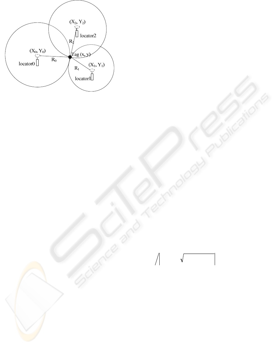
Figure 1: General Positioning in ideal environment.
2 BACKGROUND
2.1 PSO
Particle Swarm Optimization (PSO) is an
evolutionary computation technique which is based
on swarm of particle – introduced by Eberhat and
Kennedy (Kennedy and Eberhart, 1995). It has been
used to solve many optimization problems since it
was proposed (Y. Liu, Z. Qina et al., 2007). PSO is
inspired by social behaviour such as of bird flocking
and fish
schooling.
PSO starts with random population, have fitness
value to evaluate and update the population and
search for the optimum with random technique,
which is similar to other population based
optimization methods such as Genetic Algorithm
(GA) (Eberhart and Y. Shi, 1998). Particles can be
considered as agents flying through problem
dimension space looking for the solution.
General formula for PSO for representing
velocity(Vector) and position(update) can be write
in mathematical formula as:-
)(**)(***
2211
1 t
igx
t
ilx
t
ix
t
ix
xprcxprc −+−+=
+
υωυ
(1)
)(**)(***
4231
1 t
igy
t
ily
t
iy
t
iy
yprcyprc −+−+=
+
υωυ
(2)
t
i
t
ix
t
i
xx +=
++ 11
υ
(3)
t
i
t
iy
t
i
yy +=
++ 11
υ
(4)
Tt /)(*
minmaxmax
ωωωω
−−=
(5)
Where:-
- C
1
and C
2
are acceleration constants.
- r
1
, r
2
, r
3
and r
4
are random numbers between 0 – 1.
- t = current iteration.
- T = maximum numbers of iteration.
- ω= inertia weight
- P
ix
and P
iy
= Local best in X and Y direction
- P
gx
an P
gy
= Global best in X and Y direction
A key feature of PSO algorithm is social sharing
information among the neighbourhood (Y. Liu, Z.
Qina et al., 2007). When particle flies to a new
location, new problem solution is generated. Then
particle will update the knowledge with its own
previous record and with other particle record to
identify the best local position (Local Best) and the
best position for overall (Global Best). The best
fitness value (Local Best and Global Best) will be
updated based on formula:-
1
,
1
1
,
1
(6)
Where:-
-
= the best fitness value and the coordination
where the value is calculated
- = generation/iteration step
2.2 PSO-RTVIWAC
PSO-RTVIWAC was motivated by PSO-RANDIW
and PSO-TVAC. By modifying the variable used in
the standard PSO formula, PSO-RTVIWAC method
is capable of tracking and optimizing in the highly
nonlinear dynamic local positioning systems. The
variable involved can be formulated as:-
(
)
Ttr /)(**
minmaxmax5
ω
ω
ω
ω
−
−
=
(7)
(
)
Tcctcrc /)(*
minmaxmax61
−
−
∗
=
(8)
(
)
Tcctcrc /)(*
minmaxmax72
−
−
∗
=
(9)
t
i
t
ix
t
i
xkx +=
++ 11
*
υ
(10)
t
i
t
iy
t
i
yky +=
++ 11
*
υ
(11)
phiphiphik *422
2
−−−=
(12)
(
)
8
1*4 rphi
+
=
(13)
Where:-
-
,
,
are random number between 0 and
1
- k = constriction factor.
Constriction factor, k, is necessary to ensure the
convergence of the particle swarm (Y. Shi and
Eberhart, 2001, Y. Shi and Eberhart, 1998, M. Clerc
1999). It is used to prevent the particles from
exploring too far away into the search space
(Eberhart and Kennedy 1995, M. Clerc and Kennedy
2002).
UPDATING TECHNIQUE FOR PARTICLE SWARM OPTIMIZATION IN NONLINEAR DYNAMIC SYSTEMS
463
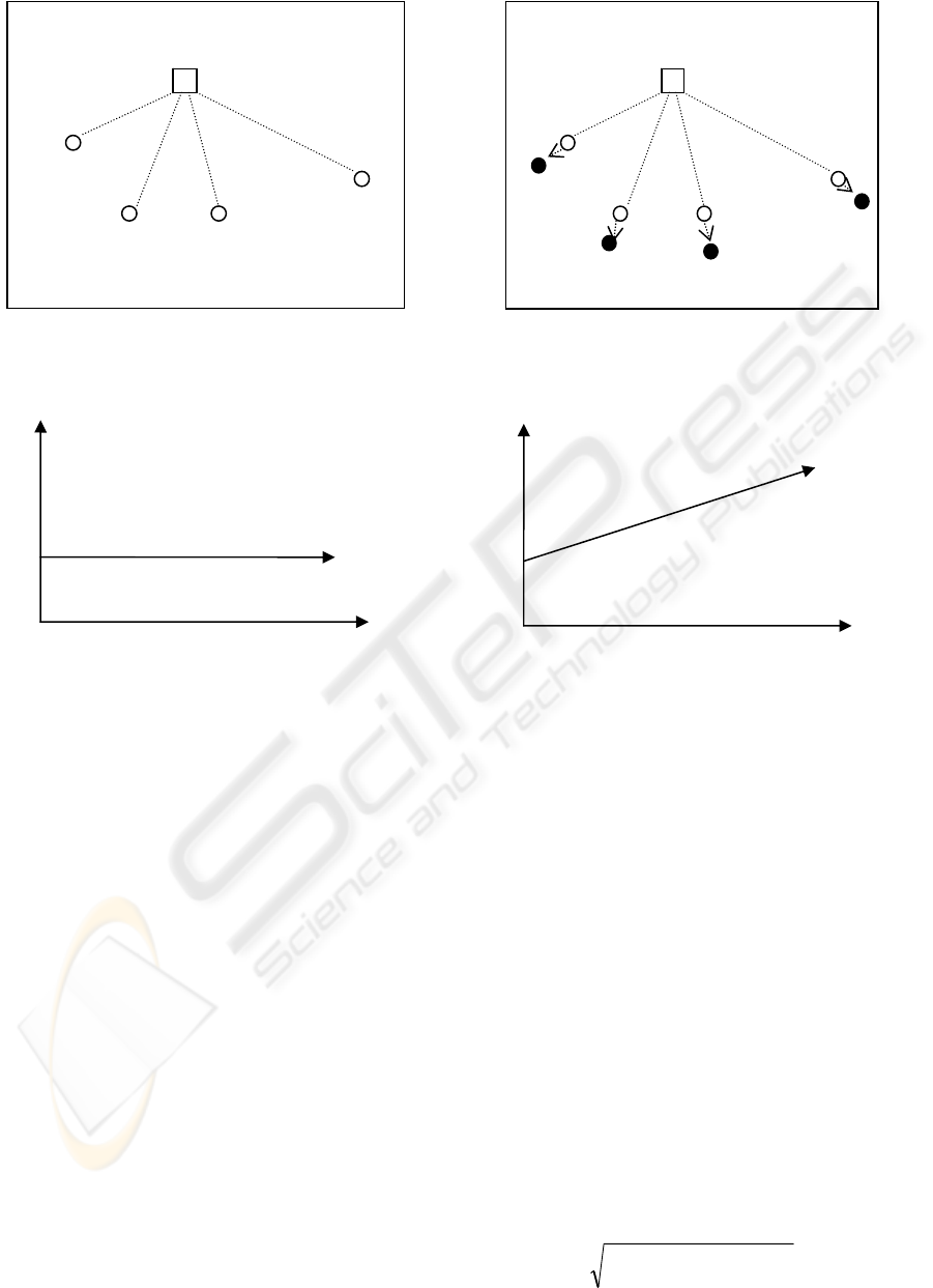
Figure 2(a): Fitness value at time t1 and t2 for PSO-
RTVIWAC.
Fitness Value
0 Times
Figure 2(b): Fitness value vs Times in PSO-RTVIWAC.
Figure 4(a) and 4(b) show the area of inertia
weight and acceleration coefficient covered by PSO-
RTVIWAC. This becomes the main idea that
outperforms three previous techniques. For updating
the knowledge (Local Best and Global Best), PSO-
RTVIWAC is using the same formula as standard
PSO. In PSO, the knowledge will not be updated
until any particle encounters a new vector location
with smaller fitness value than the value currently
stored in the particle’s memory (X. Cui, Hardin et
al., 2005).
If the current position has the smaller fitness
value then the previous, the current will be the best
and will be saved in memory. If not, then the
previous will remain as the best and kept in
memory
. Smaller fitness value means closer to the
target. If the fitness value equal to zero, this means
particle reached the target. Normally, times did not
affect the fitness value that had been achieved by the
particles. Figure 2(a) and 2(b) shows the situation of
the fitness value in PSO-RTVIWAC that is not
affected by time or iteration.
Generally, 3 steps involved in PSO-RTVIWAC.
The steps are:-
Figure 3(a): Fitness value at time t1 and t2 for proposed
updating technique.
Fitness Value
0 Times
Figure 3(b): Fitness value at time t1 and t2 for proposed
updating technique.
i. System Initialization
Locators are deployed in certain position of square
room. Target is deployed randomly Distance
between locators and target are measured.
ii. Tag Position Estimation
The program used PSO-RTVIWAV algorithm to
estimate target position. Particles swarm is
initialized with random positions and velocities. The
program then calculates the distance between
particles and locators. After that, it identifies the best
fitness function and will run again for second
iteration until the end. In every iteration, the best
fitness function will be updated based on equation
(6).
iii. Estimated Result and Error
The program completed after T. All particles
converge into global best positions where it is an
optimal solution estimated using PSO-RTVIWAC.
It will be considered as system output. Then, the
position error then is defined as:-
(14)
Locator 1 Locator 2
Target
f
1
P
1
f
4
f
2
f
3
f
1
+e P
4
P
2
P
3
f
4
+e
f
2
+e f
3
+e
Locator 3 Locator 4
Locator 1 Locator 2
Target
f
1
P
1
f
4
f
2
f
3
P
4
P
2
P
3
Locator 3 Locator 4
(
)( )
22
ypxpE
gygxp
−+−=
ICAART 2009 - International Conference on Agents and Artificial Intelligence
464

Where:-
-
gx
p
and
gy
p
are Global best in X and Y axis
- X and Y are target positions in X and Y axis.
Figure 4(a).
Figure 4(b).
3 PROPOSED UPDATING
TECHNIQUE
Particles can be considered as simple agents flying
through into problem space searching for the
solution. This solution is evaluated by a fitness
function that provides a quantitative value of the
solution’s utility (X. Cui, Hardin et al., 2005).
Fitness value for each particle will be calculated to
identify the best solution (Local Best and Global
Best) from time to time (iteration). In nonlinear
dynamic environment with numerous factors can
change the system state, smallest fitness value at
time t1 may not be the smallest value at time t2.
Figure 2(a) and 2(b) show the fitness value for PSO-
RTWIWAC. Figure 2(a) representing the fitness
value f1, f2, f3 and f4 that remain unchanged at time
t1 and time t2 even though with the existing of
numerous factor that can change the environment
state. Figure 2(b) shows the horizontal graph of
fitness value versus time.
Figure 5(a).
Figure 5(b).
Figure 5(c).
Figure 5(a), 5(b) and 5(c): Processes involved for every
step in PSO-RTVIWAC.
Third step. Estimated Results and Error
(1) The program is completed after T.
(2) Global Best position is consider as tag
p
osition
(3) Calculated estimated error Ep
Second step. Tag position estimate using PSO-
RTVIWAC
(1) Particle swarm is generated with
random position and velocity
(2) Distance between locators m and
p
articles Di are calculate
(3) For each particle, calculate optimization
fitness function Fi
(4) Update position and velocity of each
particle
First step. System initialization
(1) Locator m (m = 1 - 4) are distributed
in one room with coordinate (X
m
, Y
m
)
(2) Tag is generated at random unknown
position (x,y)
(3) Distances between locators and tag,
Rm are measured
UPDATING TECHNIQUE FOR PARTICLE SWARM OPTIMIZATION IN NONLINEAR DYNAMIC SYSTEMS
465

Compare with figure 3(a), where f
1
, f
2
, f
3
and f
4
are
the best fitness value for particle P
1
, P
2
, P
3
and P
4
at
time t
1
. To represent the factors that can change the
environment, constants value “e” will be added to
the best fitness value at time t
2
. The fitness values
now become f
1
+ e, f
2
+ e, f
3
+ e and f
4
+ e.
This mean, fitness value will constantly increase
from time to time until it is replaced by another
fitness value that has smaller value than the current
stored. Figure 3(b) representing the fitness values
constantly increase versus time. Based on this
situation, updating equation for the best fitness value
can be written as:-
1
,
1
1
,
1
(15)
Where:-
-
= the best fitness value and the
coordination where the value is calculated
- = generation/iteration step
- e = constant value vector unit between 0 - 1
The simulation will use equation (15) for
updating the fitness value. The result will then be
compared with the PSO-RTVIWAC to evaluate the
performance.
4 EXPERIMENTAL SETUP
In this section, the performance of this technique
will be compared and evaluate with PSO-
RTVIWAC. PSO-RTVIWAC is already proven to
achieve high accuracy with small number of particle
and iteration. This algorithm already outperformed
three previous techniques namely PSO-TVIW, PSO-
TVAC and PSO-RANDIW (Z. Hui, S. Ngah et al.
2008). Simulations are executed one thousand runs
to detect the target. Average positioning error will be
calculated to evaluate the performance of the
proposed method. The simulation will run under the
same condition where the PSO-RTVIWAC
outperformed the three previous techniques except
the equation for updating the particles. The numbers
of particles used in this simulation are 10, 15, 20 and
25. Iterations for all simulation are set to 20 and 50.
Dimension search space is set to 50m x 50m and the
target is randomly located within this dimension.
The results from these data will then be calculated to
produce the positioning error based on equation (15)
and average positioning error.
The average positioning error is used to
calculate the performance can be expressed as:-
()
1000
1000
1
2
,
∑
=
=
r
paveragep
EE
(16)
5 EXPERIMENTAL RESULTS
AND DISCUSSION
5.1 Number of Iteration is Set to 20
Table 1 summarized the result between PSO-
RTVIWAC and the proposed method. For the first
two results, where the numbers of particle are 10 and
15, the PSO-RTVIWAC produces better average
positioning error compared with the proposed
method. But, when the numbers of particle increased
to 20 and 25, the proposed method can achieve
better performance. It shows that, the number of
particle and total number of iteration plays a
significant role for achieving higher fitness value in
the proposed method. This can be proven when, the
simulation running with the same number of particle
but more iteration is given such as the data shown in
table 1.
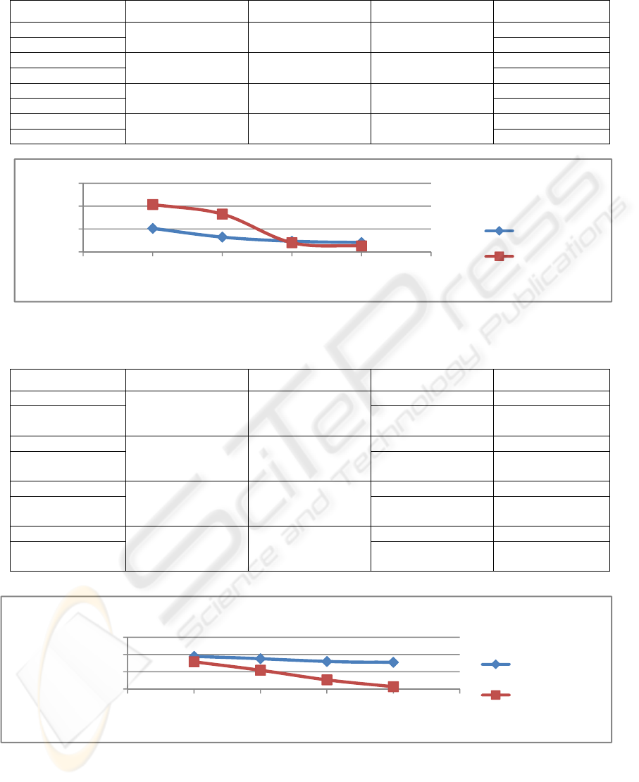
5.2 Number of Iteration is Set to 50
Table 2, summarized the result of when simulation
runs with 50 iteration. Both of simulation are
running with the value of “e” = 0.01 vector unit.
The table shows all the results achieved by the
proposed method have higher accuracy compared to
PSO-RTVIWAC. Furthermore, to produce average
positioning error that was achieved by PSO-
RTVIWAC, proposed method only needs 28 to 40
iterations. The results are shown in the bracket in
Table 2.
Further simulation then are being run to identify
the optimum value of “e” in order to produce good
result(small average positioning error). Values of
“e”
between 0.001 to 0.01 vector units are then
identified as optimum value to use in this case.
However, the value of “e” to produce better results
in other environment or problem needs more
research. It probably varies from one problem to
another.
6 CONCLUSIONS
In nonlinear dynamic systems, where a numerous of
noise and the environment keep changing from time
to time, a good algorithm is needed to find an
ICAART 2009 - International Conference on Agents and Artificial Intelligence
466
0,01
0,1
1
10
5 1015202530
AverageE
p
NumberofParticle
NumberofParticlevsAverageE
p
PSO‐RTVIWAC
Proposed
0,000001
0,0001
0,01
1
5 1015202530
AverageE
p
NumberofParticle
NumberofParticlevsAverageE
p
PSO‐RTVIWAC
Proposed
Table 1: Average Positioning Error with 20 iterations.
Number of Particle Side length (m) Number of iteration
PSO-RTVIWAC
10 50 20
1.06E-01
Proposed 1.172
PSO-RTVIWAC
15 50 20
4.40E-02
Proposed 4.45E-01
PSO-RTVIWAC
20 50 20
2.94E-02
Proposed 2.51E-02
PSO-RTVIWAC
25 50 20
2.55E-02
Proposed 1.81E-02
Figure 6: Graph Number of particle vs Average E
p
for 20 iterations.
Table 2: Average Positioning Error with 50 iterations.
Number of Particle Side length (m) Number of iteration
PSO-RTVIWAC
10 50
50 6.03E-03
Proposed 50
(40)
1.42E-03
(4.82E-03)
PSO-RTVIWAC
15 50
50 3.26E-03
Proposed 50
(30)
1.49E-04
(3.31E-03)
PSO-RTVIWAC
20 50
50 1.55E-03
Proposed 50
(30)
1.14E-05
(1.45E-03)
PSO-RTVIWAC
25 50
50 1.25E-03
Proposed 50
(28)
1.84E-06
(1.22E-03)
Figure 7: Graph Number of particle vs Average E
p
for 50 iterations.
averagep
E
,
averagep
E
,
UPDATING TECHNIQUE FOR PARTICLE SWARM OPTIMIZATION IN NONLINEAR DYNAMIC SYSTEMS
467

optimum solutions. PSO-RTVIWAC is already
proven to be a good algorithm. However, PSO-
RTVIWAC used the standard PSO algorithm
technique to update the knowledge of the particle.
By modifying the fitness value that has been used
to update the particle knowledge, the
performance
of the algorithm can be increased. This paper
proposed a new constant value to be added into
fitness value in updating equation. By applying
this constant value, the proposed technique that
used the same step as used by PSO_RTVIWAC,
can perform better. The results show that,
performance of proposed technique increased more
than 90% in average positioning error from
1.172m to 0.0181m, where as PSO-RTVIWAC
only around 75% from 0.106m to 0.0255m when
the total particle number increased from 10 to 25.
Proposed technique also needs less iteration
between 28 to 40 iterations to achieve the same
result by PSO-RTVIWAC that running with 50
iterations. The experimental results indicate this
updating technique can work effectively in
nonlinear dynamic systems.
REFERENCES
H. Zhu, S. Ngah, Y. Xu, Y. Tanabe and T. Baba “A
Random Time-varying Optimization for Local
Positioning Systems” Int. journal of Computer
Science and Network Security, Vol 8 N0 6, 2008.
X. Cui, C.T. Hardin, R.K. Ragade, T.E. Potok and A.S.
Elmaghraby “Tracking non-Optimal Solution by
Particle Swarm Optimizer” IEEE, Proc. Of Sixth Int.
Conf. on Software Engineering, Artificial Intelligent,
Networking and Parallel/Distributed Computing,
2005.
R. C. Eberhart and J. Kennedy, “A new optimizer using
particle swarm theory”, Proc. of the Sixth
International Symposium on Micro Machines and
Human Science, pp. 39-43, 1995
R. C. Eberhart and Y. Shi, “Particle swarm optimization:
developments, applications and resources”,
Proceedings of the 2001 Congress on Evolutionary
Computation, vol. 1, pp. 81-86, 2001
E. Ozcanand and C.K. Mohan, “Particle swarm
optimization: Surfing the waves,” in Proc. IEEE
Congr. Evolutionary Computation 1999, vol. 3,
Washington, DC, pp. 1944–1949, 1999.
Y. Shi and R. C. Eberhart, “A modified particle swarm
optimizer,” in Proc. IEEE Int. Conf. Evolutionary
Computation, pp. 69–73, 1998
R. C. Eberhart and Y. Shi, “Comparing Inertia Weights
and Constriction Factors in Particle Swarm
Optimization,” Congress on Evolutionary
Computing, vol. 1, pp. 84-88, 2000.
R. C. Eberhart and Y. Shi, “Comparison between genetic
algorithms and particle swarm optimization,” The
7th Annual Conference on Evolutionary
Programming, pp. 611-615, 1998.
M. Clerc, “The swarm and the queen: towards a
deterministic and adaptive particle swarm
optimization,” Proc. CEC 1999, Washington, DC, pp
1951-1957, 1999.
Y. Liu, Z. Qina, Z. Shi, J. Lu “Center Particle Swarm
Optimization” Neurocomputing 70 (2007) pp. 672 -
679. www.sciencedirect.com.
R. C. Eberhart and Y. Shi, “Tracking and optimizing
dynamic systems with particle swarms,” in Proc.
IEEE Congr. Evolutionary Computation 2001,
Seoul, Korea, pp. 94–97, 2001
M. Clerc and J. Kennedy, “The particle swarm:
Explosion, stability, and convergence in a multi-
dimensional complex space,” IEEE Transactions on
Evolutionary Computation, pp. 58-73, 2002
ICAART 2009 - International Conference on Agents and Artificial Intelligence
468
