
STATE AGGREGATION FOR REINFORCEMENT LEARNING
USING NEUROEVOLUTION
Robert Wright and Nathaniel Gemelli
Air Force Research Lab, Information Directorate, 525 Brooks Rd., Rome, 13441, U.S.A.
Keywords:
Reinforcement learning, NeuroEvolution, Evolutionary algorithms, State aggregation.
Abstract:
In this paper, we present a new machine learning algorithm, RL-SANE, which uses a combination of neuroevo-
lution (NE) and traditional reinforcement learning (RL) techniques to improve learning performace. RL-SANE
is an innovative combination of the neuroevolutionary algorithm NEAT(Stanley, 2004) and the RL algorithm
Sarsa(λ)(Sutton and Barto, 1998). It uses the special ability of NEAT to generate and train customized neural
networks that provide a means for reducing the size of the state space through state aggregation. Reducing
the size of the state space through aggregation enables Sarsa(λ) to be applied to much more difficult problems
than standard tabular based approaches. Previous similar work in this area, such as in Whiteson and Stone
(Whiteson and Stone, 2006) and Stanley and Miikkulainen (Stanley and Miikkulainen, 2001), have shown
positive and promising results. This paper gives a brief overview of neuroevolutionary methods, introduces
the RL-SANE algorithm, presents a comparative analysis of RL-SANE to other neuroevolutionary algorithms,
and concludes with a discussion of enhancements that need to be made to RL-SANE.
1 INTRODUCTION
Recent progress in the field of neuroevolution has
lead to algorithms that create neural networks to solve
complex reinforcement learning problems (Stanley,
2004). Neuroevolution refers to technologies which
build and train neural networks through an evolution-
ary process such as a genetic algorithm. Neuroevolu-
tionary algorithms are attractive in that they are able
to automatically generate neural networks. Manual
engineering, domain expertise, and extensive training
data are no longer necessary to create effective neu-
ral networks. One problem with these algorithms is
that they rely heavily on the random chance of muta-
tion operators to produce networks of sufficient com-
plexity and train them with the correct weights to
solve the problem at hand. As a consequence, neu-
roevolutionary methods can be slow or unable to con-
verge to a good solution. Traditional reinforcement
learning (RL) algorithms on the other hand take cal-
culated measures to improve their policies and have
been shown to converge very quickly. However, RL
algorithms rely on costly Q-tables or predetermined
function approximators to enable them to work on
complex problems. A hybrid of the two technologies
has the potential to provide an algorithm with the ad-
vantages of both.
We present a new machine learning algorithm,
which combines neuroevolution and traditional re-
inforcement learning techniques in a unique way.
RL-SANE
1
, Reinforcement Learning using State Ag-
gregation via Neuroevolution, is an algorithm de-
signed to take full advantage of neuroevolutionary
techniques to abstract the state space into a more
compact representation for a reinforcement learner
that is designed to exploit its knowledge of that
space. We have combined a neuroevolutionary algo-
rithm developed by Stanley and Miikkulainen called
NEAT(Stanley and Miikkulainen, 2001) with the re-
inforcement learning algorithm Sarsa(λ)(Sutton and
Barto, 1998). Neural networks serve as excellent
function approximators to abstract knowledge while
reinforcement learners are inherently good at ex-
ploring and exploiting knowledge. By utilizing the
1
It should be noted that RL-SANE is not related to the
SANE algorithm(Moriarty and Miikkulainen, 1997), Sym-
biotic Adaptive NeuroEvolution. SANE is a competing
neuroevolutionary algorithm with NEAT that uses a coop-
erative process to evolve NNs.
45
Wright R. and Gemelli N. (2009).
STATE AGGREGATION FOR REINFORCEMENT LEARNING USING NEUROEVOLUTION.
In Proceedings of the International Conference on Agents and Artificial Intelligence, pages 45-52
DOI: 10.5220/0001658800450052
Copyright
c
SciTePress

strengths of both of these methods we have created
a robust and efficient machine learning approach in
RL-SANE.
The rest of the paper is organized as follows. Sec-
tion 2 will give an overview of the problem on which
are working and other state aggregation approaches
that have been done. Section 3 will provide a full de-
scription and discussion on the RL-SANE algorithm.
In sections 4.3 and 4.4 we will provide experimen-
tal results for RL-SANE. Section 4.3 provides in-
sight into how the β parameter affects performance
and how it can be determined. Section 4.4 completes
the analysis with a comparison of RL-SANE’s perfor-
mance versus a standard neuroevolutionary approach,
NEAT, on two standard benchmark problems. Finally,
section 5 will highlight our future work.
2 BACKGROUND
The state aggregation problem for machine learning
has started to gain more momentum over the past
decade. Singh et al. used soft state aggregation meth-
ods in (Singh et al., 1995) and discussed how impor-
tant compact representations are to learning methods.
Stanley and Miikkulainen (Stanley and Miikkulainen,
2002) discuss using neural networks for state aggre-
gation and learning and demonstrated promising re-
sults for real-world applications. Further improve-
ments to neuroevolutionary approaches were done in
Siebel et al. in (Siebel et al., 2007) and combina-
tions of neuroevolution and reinforcement learning
were studied in Whiteson and Stone in (Whiteson
and Stone, 2006). Neuroevolution has been shown
to be one of the strongest methods for solving com-
mon benchmarking problems, such as pole-balancing
(Stanley and Miikkulainen, 2002). This section will
highlight neuroevolution and describe the NEAT al-
gorithm which we use as a benchmark to compare our
work against.
2.1 Neuroevolution
Neuroevolution (NE) (Stanley and Miikkulainen,
2001) is a technology that encompasses techniques
for the artificial evolution of neural networks. Tra-
ditional work in neural networks used static neural
networks that were designed by subject matter ex-
perts and engineers. This method showed the power
of neural networks in being able to model and learn
non-linear functions. However, the static nature of
these structures limited their scope and applicability.
More recent advances in the field of neuroevolution
have shown that it is possible to build and configure
these networks dynamically through the use of special
mutation operators in a genetic algorithm (GA) (Stan-
ley, 2004). These advances have made it possible
to automatically generate and train special purpose
neural networks for solving difficult multi-parameter
problems. We recognize similar work in this area as
in Siebel et al. (Siebel et al., 2007), Stanley et al.
(Stanley and Miikkulainen, 2001), and Whiteston and
Stone (Whiteson and Stone, 2006) exists and below
we describe one such algorithm, NEAT.
2.2 NEAT
NeuroEvolution of Augmenting Topologies (NEAT)
is a neuroevolutionary algorithm and framework
which uses a genetic algorithm to evolve populations
of neural networks. It is a neuroevolutionary algo-
rithm that evolves both the network topology and
weights of the connections between the nodes in the
network(Stanley and Miikkulainen, 2002). The au-
thors, Stanley et al., found that by evolving both the
network topology and the connection weights, they
solved typical RL benchmark problems several times
faster than competing RL algorithms(Stanley and Mi-
ikkulainen, 2001) with significantly less system re-
sources. The algorithm starts with a population of
simple perceptron networks and gradually, through
the use of a genetic algorithm (GA), builds more com-
plex networks with the proper structure to solve a
problem. It is a bottom-up approach which takes
advantage of incremental improvements to solve the
problem. The results are networks that are automat-
ically generated, not overly complicated in terms of
structure, and custom tuned for the problem at hand.
Two of the most powerful aspects of NEAT
which allow for such good benchmark perfor-
mance and proper network structure are complexifi-
cation(Stanley, 2004) and speciation(Stanley and Mi-
ikkulainen, 2002). Complexification, in this context,
is an evolutionary process of constructing neural net-
works through genetic mutation operators. These ge-
netic mutation operators are: modify weight, add link,
and add node (Stanley, 2004). Speciation is a method
for protecting newly evolved neural network struc-
tures (specie) into the general population, and prevent
them from having to compete with more optimized
species (Stanley, 2004). This is important to preserve
new (possibly helpful) structures with less optimized
network weights.
ICAART 2009 - International Conference on Agents and Artificial Intelligence
46
3 RL-SANE
RL-SANE is the algorithm we have developed which
is a combination of NEAT and a RL algorithm
(Sarsa(λ)(Sutton and Barto, 1998)). This combina-
tion was chosen because neural networks have been
shown to be effective at reducing the complexities of
state spaces for RL algorithms(Tesauro, 1995). NEAT
was chosen as a way for providing the neural net-
works because it is able to build and train networks
automatically and effectively. Sarsa(λ) was chosen
because of its performance characteristics. Any NE
algorithm that automatically builds neural networks
can be substituted for NEAT and any RL algorithm
can be substituted in Sarsa(λ)’s place, and RL-SANE
should still function.
RL-SANE uses NE to evolve neural networks
which are bred specifically to interpret and aggregate
state information. NEAT networks take the raw per-
ception values and filter the information for the RL
algorithm by aggregating inputs together which are
similar with respect to solving the problem
2
. This re-
duces the state space representation and enables tradi-
tional RL algorithms, such as Sarsa(λ), to function on
problems where the raw state space of the problem is
too large to explore. NEAT is able to create networks
which accomplish the filtering by evolving networks
that improve the performance of Sarsa(λ) in solving
the problem. Algorithm 1 provides the pseudo code
for RL-SANE and describes the algorithm in greater
detail.
What differentiates RL-SANE from other algo-
rithms which use NE to do learning, such as in NEAT,
is that RL-SANE separates the two mechanisms that
perform the state aggregation and policy iteration.
Previous NE algorithms(Stanley and Miikkulainen,
2001)(Whiteson and Stone, 2006) use neural net-
works to learn a function which not only encompasses
a solution to the state aggregation problem, but the
policy iteration problem as well. We believe this over-
burdens the networks and increases the likelihood of
“interference”(Carreras et al., 2002). In this context,
“interference” is the problem of damaging one aspect
of the solution while attempting to fix another. RL-
SANE, instead, only uses the neural networks to per-
form the state aggregation and uses Sarsa(λ) to per-
form the policy iteration which reduces the potential
impact of interference.
The purpose of the neural networks created by
the NEAT component is to filter the state space for
2
“With respect to the problem” in this paper refers to
groupings made by NEAT which improve Sarsa(λ)’s ability
to solve the problem, not necessarily the grouping of similar
perceptual values.
Algorithm 1 RL-SANE(S,A,p,m
n
,m
l
,m
r
,g,e,α,β,γ,λ,ε)
1: //S: set of all states, A: set of all actions
2: //p: population size, m
n
: set of all states, m
l
: link mutation rate
3: //m
r
: link removal mutation rate, g: number of generations
4: //e: number of episodes per generation, α: learning rate
5: //β: state bound, γ: discount factor, λ: eligibility decay rate
6: //ε: ε-Greedy probability
7: P[] ← INIT-POPULATION(S,p) // create a new population P of random
networks
8: Q
t
[] ← new array size p // initialize array of Q tables
9: for i ← 1 to g do
10: for j ← 1 to p do
11: N,Q[] ← P[ j], Q
t
[ j] // select network and Q table
12: if Q[] = null then
13: Q[]←new array size β // create a new Q table
14: end if
15: for k ← 1 to e do
16: s,s
0
←null, INIT-STATE(S) // initialize the state
17: repeat
18: s
0
id
←INT-VAL(EVAL-NET(N,s
0
)*β) // determine the
state id
19: with-prob(ε) a
0
←RANDOM(A) // ε-Greedy action se-
lection
20: else a
0
←argmax
l
Q[s
0
id
,l]
21: if s6=null then
22: SARSA(r,a,a
0
,λ,γ,α,Q[],s
id
,s
0
id
)//update Q table
23: end if
24: s
id
,s,a←s
0
id
,s
0
,a
0
25: r,s
0
←TAKE-ACTION(a
0
)
26: N. f itness←N. f itness+r // update the fitness of the net-
work
27: until TERMINAL-STATE(s)
28: end for
29: Q
t
[ j]←Q[] // update array of Q tables
30: end for
31: P
0
[],Q
0
t
← new arrays size p // array for next generation
32: for j←1 to p do
33: P
0
[ j],Q
0
t
[ j]←BREED-NET(P[],Q
t
[]) // make a new network and
Q table based on parents
34: with-probability m
n
: ADD-NODE-MUTATION(P
0
[ j])
35: with-probability m
l
: ADD-LINK-MUTATION(P
0
[ j])
36: with-probability m
r
: REMOVE-LINK-MUTATION(P
0
[ j])
37: end for
38: P[],Q
t
[]←P
0
[],Q
0
t
[]
39: end for
Sarsa(λ). They do this by determining if different
combinations of perceptual inputs should be consid-
ered unique states with respect to the problem. This is
done by mapping the raw multi-dimensional percep-
tual information onto a single dimensional continuum
which is a real number line in the range [0..1]. The
state bound parameter, β, divides the continuum into
a specified number of discrete areas and provides an
upper bound on the number of possible states there are
in the problem. All points on the continuum within
a single area are considered to be the same state by
RL-SANE and are labeled with a unique state iden-
tifier. The output of the neural networks, given a set
STATE AGGREGATION FOR REINFORCEMENT LEARNING USING NEUROEVOLUTION
47

of perception values, is the state identifier of the area
the perception values map on to the continuum. RL-
SANE uses this state identifier as input to the Sarsa(λ)
RL component as an index into its Q-table. The Q-
table is used to keep track of values associated with
taking different actions in specific states. The net-
works which are best at grouping perception values
that are similar with respect to solving the problem
will enable Sarsa(λ) to learn how to solve the prob-
lem more effectively.
Sarsa(λ) provides a fitness metric for each net-
work to NEAT by reporting the aggregate reward it
received in attempting to learn the problem. This
symbiotic relationship provides NEAT with a fitness
landscape for discovering better networks. This also
provides Sarsa(λ) with a mechanism for coping with
complex state spaces, via reducing complexity. Re-
ducing the complexity of the state space makes the
problem easier to solve by reducing the amount of ex-
ploration needed to calculate a good policy. It also
needs to be stated that Q-tables persist with the neural
networks they are trained on throug out the evolution
of the networks. When crossover occurs in NEAT’S
GA, the Q-table of the primary parent gets passed on
to the child neural network.
Selection of an appropriate or optimal state bound
(β) is of great importance to the performance of the al-
gorithm. If the selected state bound is too small, sets
of perception values that are not alike with respect to
the problem will be aggregated into the same state.
This may hide relevant information from Sarsa(λ) and
prevent it from finding the optimal, or even a good,
policy. If the state bound is too large, then percep-
tion sets that should be grouped together may map
to different states. This forces Sarsa(λ) to experi-
ence and learn more states than are necessary. Ef-
fectively, this slows the rate at which Sarsa(λ) is able
to learn a good policy because it is experiencing and
exploring actions for redundant states, causing bloat.
Bloat makes the Q-tables larger than necessary, in-
creasing the memory footprint of the algorithm. Im-
proper state bound values have adverse effects on the
performance of RL-SANE. Section 4.3 provides some
insight into how varying β values affects RL-SANE’s
performance and gives guidance on how to set β.
We recognize that RL-SANE is not the first al-
gorithm that attempts to pair NE techniques with
a traditional RL algorithm. NEAT+Q by Whiteson
and Stone (Whiteson and Stone, 2006) combines Q-
learning (Watkins and Dayan, 1992) with NEAT in a
different way than RL-SANE. In NEAT+Q the neural
networks are meant to output literal Q-values for all
the actions available in the given state. The networks
are trained on-line to produce the correct Q-values via
the Q-learning update function and the use of back-
propagation (Rumelhart et al., 1988). We attempted
to use NEAT+Q in our analysis of RL-SANE but we
were unable to duplicate the results found in (White-
son and Stone, 2006), so we are unable to present a
comparison. Also, both RL-SANE and NEAT+Q are
not easily adapted to work on problems with continu-
ous action spaces, whereas NEAT is. RL-SANE and
NEAT+Q both make discrete choices of actions.
4 EXPERIMENTS
This section describes our experimental setup for an-
alyzing the performance of the RL-SANE algorithm.
In our experiments we compare RL-SANE’s per-
formance on two well known benchmark problems,
mountain car (Boyan and Moore, 1995) and double
inverted pendulum (Gomez and Miikkulainen, 1999),
against itself with varying β values and against that of
NEAT. NEAT was chosen as the benchmark algorithm
of comparison because it is a standard for neuroevo-
lutionary algorithms (Whiteson and Stone, 2006).
Both of the algorithms for our experiments were
implemented using Another NEAT Java Implemen-
tation (ANJI)(James and Tucker, 2004). ANJI is a
NEAT experimentation platform based on Kenneth
Stanley’s original work written in Java. ANJI includes
a special mutation operator not included in the orig-
inal NEAT algorithm that randomly prunes connec-
tions in the neural networks. This mutation operator is
beneficial in that it attempts to remove redundant and
excess structure from the neural networks. The prune
operator was enabled and used by each algorithm in
our experiments. For our experiments we used the
default parameters for ANJI with the exceptions that
we disallowed recurrent networks and we limited the
range of the weight values to be [-1..1]. We disal-
lowed recurrency to reduce their overall complexity
of the networks and we bounded the link weights so
the calculation of the state from the output signal is
trivial.
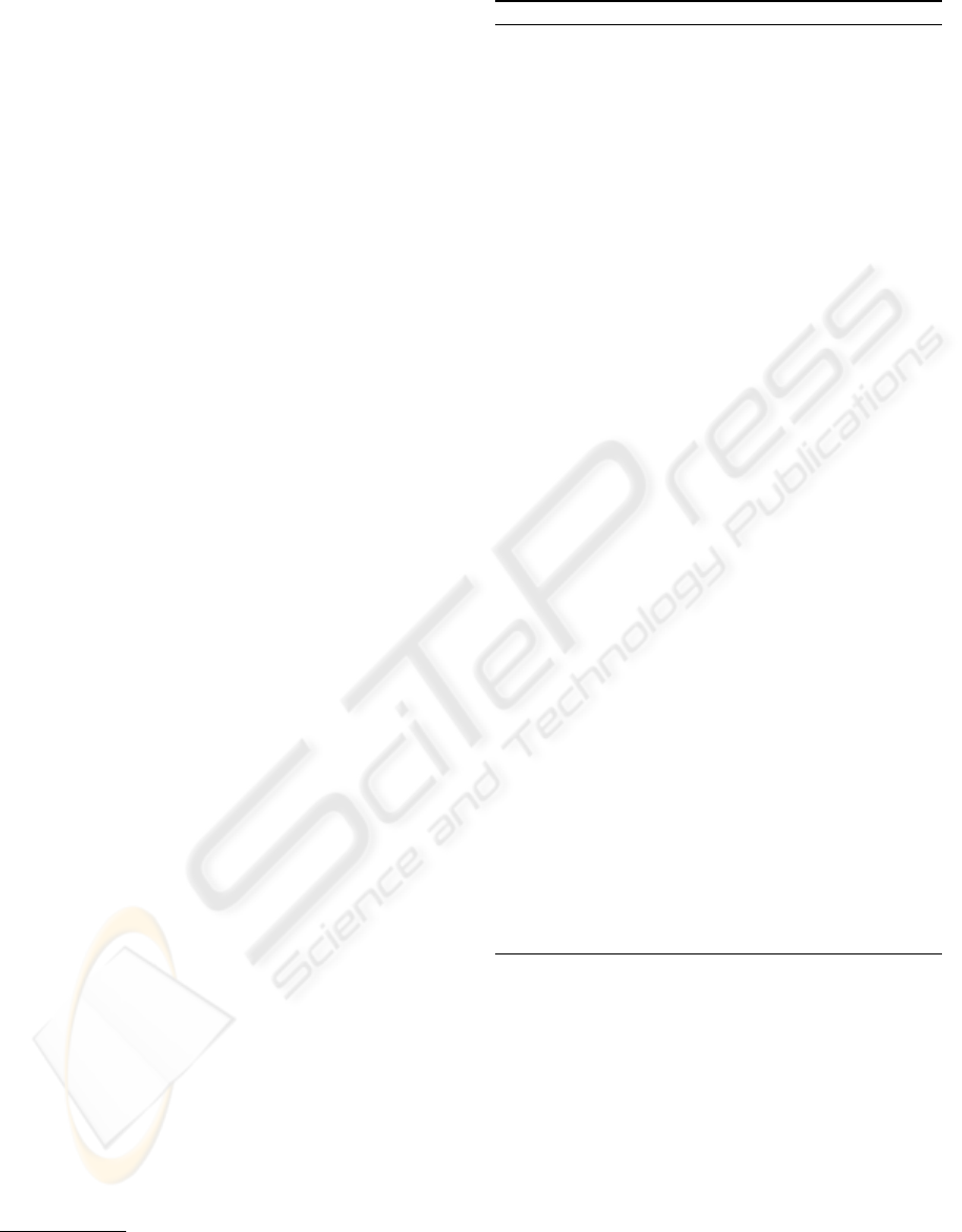
4.1 Mountain Car
The mountain car problem (Boyan and Moore, 1995)
is a well known benchmark problem for reinforce-
ment learning algorithms. In this problem a car begins
somewhere in the basin of a valley, of which it must
escape. See Figure 1 for an illustration of the prob-
lem. Unfortunately, the car’s engine is not powerful
enough to drive directly up the hill from a standing
start at the bottom. To get out of the valley and reach
the goal position the car must build up momentum
ICAART 2009 - International Conference on Agents and Artificial Intelligence
48
from gravity by driving back and forth, up and down
each side of the valley.
For this problem the learner has two perceptions:
the position of the car, X, and the velocity of car, V .
Time is discretized into time steps and the learner is
allowed one of two actions, drive forward or back-
ward, during each time step. The only reward the
learner is given is a value of -1 for each time step
of the simulation in which it has not reached the
goal. Because the RL algorithms are seeking to max-
imize aggregate rewards, this negative reward gives
the learner an incentive to learn a policy which will
reach the goal in as few time steps as possible.
The mountain car problem is a challenging prob-
lem for RL algorithms because it has continuous in-
puts. The problem has an almost infinite number of
states if each set of distinct set perceptual values is
taken to be a unique state. It is up to the learner or the
designer of the learning algorithm to determine under
what conditions the driver of the car should consider
a different course of action.
In these experiments the populations of neural net-
works for all of the algorithms have two input nodes,
one for X and one for V , which are given the raw
perceptions. NEAT networks have three output nodes
(one for each direction the car can drive plus coasting)
to specify the action the car should take. RL-SANE
networks have a single output node which is used to
identify the state of the problem.
Individual episodes are limited to 2500 time steps
to ensure evaluations will end. Each algorithm was
recored for 25 different runs using a unique random
seed for the GA. The same set of 25 random seeds
were used in evaluating all three algorithms. Runs
were composed of 100 generations in which each
member of the population was evaluated over 100
episodes per generation. The population size for the
GA was set to 100 for every algorithm. Each episode
challenged the learner with a unique instance of the
problem from a fixed set that starts with the car in a
different location or having a different velocity. By
varying the instances over the episodes we helped en-
sure the learners were solving the problem and not
just a specific instance.
4.2 Double Inverted Pendulum
Balancing
The double inverted pendulum balancing problem
(Gomez and Miikkulainen, 1999) is a very difficult
RL benchmark problem. See figure 1 for an illustra-
tion of this problem. In this problem the learner is
tasked with learning to balance two beams of differ-
ent mass and length attached to a cart that the learner
Figure 1: These figures illustrate the two RL benchmark
problems, (Above)mountain car and (Below) double in-
verted pendulum balancing.
can move. The learner has to prevent the beams from
falling over without moving the cart past the barriers
which restrict the cart’s movement. If the learner is
able to prevent the beams from falling over for a spec-
ified number of time steps the problem is considered
solved.
The learner is given six perceptions as input: X is
the position of the cart, X
0
is the velocity of the cart, θ
1 and 2 are the angles of the beam, and θ
0
1 and 2 are
the angular velocities of the beams. At any given time
step the learner can do one of the following actions:
push the cart left, push the cart right, or not push the
cart at all.
Like the mountain car problem, this problem is
very difficult for RL algorithms because the percep-
tion inputs are continuous. This problem is much
more difficult in that it has three times as many per-
ceptions giving it a dramatically larger state space. In
these experiments each algorithm trains neural net-
works that have six input nodes, one for each per-
ception. NEAT has three output nodes, one for each
action. RL-SANE only has one output node for the
identification of the current state.
In this set of experiments the algorithms were
tasked with creating solutions that could balance the
pendulum for 100000 time steps. Each algorithm
was evaluated over 25 different runs where the ran-
dom seed was modified. Again, the same set of ran-
dom seeds was used in evaluating all three algorithms.
Runs were composed of 200 generations with a popu-
lation size of 100. In each generation, every member
of the population was evaluated on 100 different in-
stances of the inverted pendulum problem. The aver-
age number of steps the potential solution was able to
balance the pendulum over the set of 100 determined
its fitness.
STATE AGGREGATION FOR REINFORCEMENT LEARNING USING NEUROEVOLUTION
49
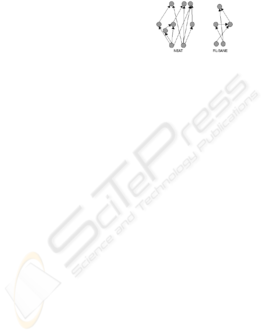
4.3 Changing the Size of State Bounds
Figure 3 shows convergence graphs for RL-SANE us-
ing varying β values, the state bound, on both bench-
mark problems. The graphs show the average number
of steps the most fit members of the population were
able to either solve the mountain car problem in or
balance the beams for. For the mountain car experi-
ments fewer steps taken is better and for the double
inverted pendulum problem the more steps the beams
were balanced for the better. For these experiments
we varied the β parameter from equal to the number of
actions available in the problems (3) up to 1000. The
purpose of these experiments is to show how varying
the β parameter affects the performance of the RL-
SANE algorithm.
When β is set equal to the number of actions avail-
able the neural networks do all the work. They have
to identify the state and determine the policy. All the
Sarsa(λ) component is doing is choosing which ac-
tion best corresponds with the output of the network.
What is interesting is if you compare the correspond-
ing graphs from figure 3 and figure 4 when β equals 3
the performance of RL-SANE is still better than that
of NEAT. This is interesting because the networks
from both algorithms are both performing the same
function and are effectively produced by the same al-
gorithm, NEAT. The reason RL-SANE has an advan-
tage over standard NEAT in this case is that Sarsa(λ)
helps RL-SANE choose the best action corresponding
with the network output whereas the actions in NEAT
are fixed to specific outputs. This result shows that
RL-SANE’s performance on problems with discrete
actions spaces is going to be as good or better than
that of NEAT if β is set to a small value. Smaller
β values preferred because they limit the size of the
Q-tables RL-SANE requires and it improves the solu-
tion’s generality.
As β is increased from 3 to larger values we see
the performance of RL-SANE improve, but once the
value of β exceeds a certain value the performance of
RL-SANE begins to drop. The performance increase
can be attributed to a burden shift from the NN to the
RL component. Sarsa(λ) is much more efficient at
performing the policy iteration than the NEAT com-
ponent. Eventually the performance degrades because
the NN(s) begin to identify redundant states as being
different, which increases the amount of experience
necessary for the RL component to learn. This behav-
ior is what we expected and shows that there might
convex fitness landscape for β values. A convex fit-
ness landscape would mean that proper β values could
be found by a simple hill climbing algorithm instead
of having to specify them a priori.
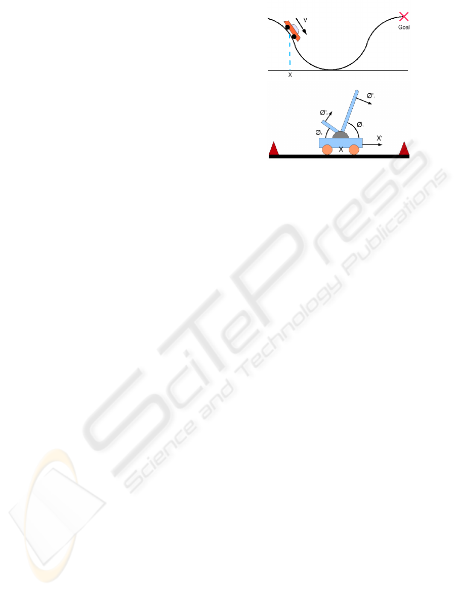
Figure 2: This figure shows the structure of typical solution
neural networks for the mountain car problem. The β value
for RL-SANE was set to 50.
It is also interesting that the double inverted pen-
dulum problem runs are more sensitive to the value of
β than the mountain car problem runs are. We are not
certain of the reason for this behavior. This requires
further investigation, and we hypothesize that more
complex problems will be more sensitive to β value
selection.
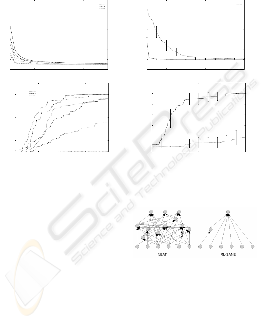
4.4 NEAT Comparison
Figure 4 show convergence graphs comparing the RL-
SANE to NEAT on the benchmarks. The error bars
on the graphs indicate 95% confidence intervals over
the entire set of experiments to show statistical signif-
icance of the results. As can be seen from the charts
the RL-SANE algorithm is able to converge to the fi-
nal solution in far fewer generations and with a greater
likelihood of success than NEAT in both sets of exper-
iments. NEAT is only able to solve the entire double
inverted pendulum problem set in just 2 of the 25 runs
of experiments. The performance difference between
RL-SANE and NEAT increases dramatically from the
mountain car to double inverted pendulum problem
which implies that RL-SANE may scale to more dif-
ficult problems better than NEAT.
Figures 2 and 5 show the structure of typical so-
lution NN(s) for both RL-SANE and NEAT on both
problems. In both figures the RL-SANE networks are
much less complex than the NEAT networks. These
results are not very surprising in that the RL-SANE
networks are performing a less complicated function,
state aggregation. NEAT networks need to perform
their own version of state abstraction and policy itera-
tion. The fact the RL-SANE networks do not need to
be as complicated as NEAT networks explains why
RL-SANE is able to perform better than NEAT on
these benchmarks. If the NN’s do not need to be as
complex they have a greater likelihood of being pro-
duced by the GA earlier in the evolution. This result
also supports our belief that RL-SANE will scale bet-
ter to more complex problems than standard NEAT.
ICAART 2009 - International Conference on Agents and Artificial Intelligence
50
0
100
200
300
400
500
600
700
0 5 10 15 20
Steps
Generations
Beta 3
Beta 5
Beta 10
Beta 50
Beta 100
Beta 1000
0
20000
40000
60000
80000
100000
120000
0 50 100 150 200
Steps
Generations
Beta 3
Beta 5
Beta 10
Beta 50
Beta 100
Beta 1000
Figure 3: Shows the performance of the RL-SANE algo-
rithm using varying β values on the mountain car (Above)
and the double inverted pendulum (Below) problems.
5 FUTURE WORK
5.1 State Bounding
RL-SANE, in its current form, depends on the state
bound parameter, β, for the problem to be known a
priori. For an algorithm that is intended to reduce or
eliminate the need for manual engineering or domain
expertise. In many cases, this a prior knowledge is
not available. Much of our future research effort will
be placed on developing a method for automatically
deriving the state bound value. For reasons stated
in section 3 and 4.3 we believe that the problem of
finding good β values has a convex landscape that a
hill climbing algorithm, such as a GA, can properly
search. In our future research we will explore dif-
ferent methods for calculating β automatically, even
perhaps during the evolution of solving the problem.
5.2 RL-SANE Scaling
Our background research on RL and methods for han-
dling large state spaces revealed a lack of work done
0
50
100
150
200
250
300
350
0 10 20 30 40 50
Steps
Generations
RL-SANE
NEAT
0
20000
40000
60000
80000
100000
120000
0 50 100 150 200
Steps
Generations
RL-SANE
NEAT
Figure 4: Shows the performance of the RL-SANE al-
gorithm compared to that of NEAT on the mountain car
(Above) and the double inverted pendulum (Below) prob-
lems. The RL-SANE runs used a β value of 50 for the
mountain car problem and 10 for the double inverted pen-
dulum problem.
Figure 5: This figure shows the structure of typical solution
neural networks for the double inverted pendulum problem.
The β value for RL-SANE was set to 10.
to examine just how well these methods scale towards
ever more complicated problems. This is surpris-
ing considering that there are so many algorithms de-
signed to improve the scaling of RL algorithms to-
wards larger state spaces. In the works that we have
examined, the authors generally chose a single in-
stance of a problem that was difficult or impossible
for existing algorithms. They then showed how their
algorithms could solve that instance. In our future
work we intend to perform experiments that stress and
STATE AGGREGATION FOR REINFORCEMENT LEARNING USING NEUROEVOLUTION
51

examine the scalability of RL-SANE and the other
neuroevolutionary based algorithms, such as NEAT,
NEAT+Q, and EANT (Siebel et al., 2007), to find out
just how far these algorithms can be pushed.
6 CONCLUSIONS
In this paper, we have introduced the RL-SANE al-
gorithm, explored its performance under varying β
values, and provided a comparative analysis to other
neuroevolutionary learning approaches. Our exper-
imental results have show that RL-SANE is able to
converge to good solutions over less iterations and
with less computational expense than NEAT even
with naively specified β values. The combination of
neuroevolutionary methods to do state aggregation for
traditional reinforcement learning algorithms appears
to have real merit. RL-SANE is, however, dependent
on the β parameter which must be calculated a priori.
We have shown the importance of the derivation of
proper β parameters and suggested finding methods
for automating the derivation of β as a direction for
future research.
Building off of what has been done by previ-
ous neuroevolutionary methods, we have found that
proper decomposition of the problem into state aggre-
gation and policy iteration is relevant. By providing
this decomposition, RL-SANE should be more appli-
cable to higher complexity problems than existing ap-
proaches.
REFERENCES
Boyan, J. A. and Moore, A. W. (1995). Generalization in re-
inforcement learning: Safely approximating the value
function. In Tesauro, G., Touretzky, D. S., and Leen,
T. K., editors, Advances in Neural Information Pro-
cessing Systems 7, pages 369–376, Cambridge, MA.
The MIT Press.
Carreras, M., Ridao, P., Batlle, J., Nicosebici, T., and Ur-
sulovici, Z. (2002). Learning reactive robot behav-
iors with neural-q learning. In IEEE-TTTC Interna-
tional Conference on Automation, Quality and Test-
ing, Robotics. IEEE.
Gomez, F. J. and Miikkulainen, R. (1999). Solving non-
markovian control tasks with neuro-evolution. In IJ-
CAI ’99: Proceedings of the Sixteenth International
Joint Conference on Artificial Intelligence, pages
1356–1361, San Francisco, CA, USA. Morgan Kauf-
mann Publishers Inc.
James, D. and Tucker, P. (2004). A comparative analysis
of simplification and complexification in the evolution
of neural network topologies. In Proceedings of the
2004 Conference on Genetic and Evolutionary Com-
putation. GECCO-2004.
Moriarty, D. E. and Miikkulainen, R. (1997). Forming neu-
ral networks through efficient and adaptive coevolu-
tion. Evolutionary Computation, 5:373–399.
Rumelhart, D. E., Hinton, G. E., and Williams, R. J.
(1988). Learning representations by back-propagating
errors. Neurocomputing: foundations of research,
pages 696–699.
Siebel, N. T., Krause, J., and Sommer, G. (2007). Efficient
Learning of Neural Networks with Evolutionary Algo-
rithms, volume Volume 4713/2007. Springer Berlin /
Heidelberg, Heidelberg, Germany.
Singh, S. P., Jaakkola, T., and Jordan, M. I. (1995). Re-
inforcement learning with soft state aggregation. In
Tesauro, G., Touretzky, D., and Leen, T., editors,
Advances in Neural Information Processing Systems,
volume 7, pages 361–368. The MIT Press.
Stanley, K. O. (2004). Efficient evolution of neural networks
through complexification. PhD thesis, The University
of Texas at Austin. Supervisor-Risto P. Miikkulainen.
Stanley, K. O. and Miikkulainen, R. (2001). Evolving neu-
ral networks through augmenting topologies. Techni-
cal report, University of Texas at Austin, Austin, TX,
USA.
Stanley, K. O. and Miikkulainen, R. (2002). Efficient
reinforcement learning through evolving neural net-
work topologies. In GECCO ’02: Proceedings of the
Genetic and Evolutionary Computation Conference,
pages 569–577, San Francisco, CA, USA. Morgan
Kaufmann Publishers Inc.
Sutton, R. S. and Barto, A. G. (1998). Reinforcement Learn-
ing: An Introduction (Adaptive Computation and Ma-
chine Learning). The MIT Press.
Tesauro, G. (1995). Temporal difference learning and td-
gammon. Commun. ACM, 38(3):58–68.
Watkins, C. J. C. H. and Dayan, P. (1992). Q-learning. Ma-
chine Learning, 8(3-4):279–292.
Whiteson, S. and Stone, P. (2006). Evolutionary function
approximation for reinforcement learning. Journal of
Machine Learning Research, 7:877–917.
ICAART 2009 - International Conference on Agents and Artificial Intelligence
52
