
A KNOWLEDGE-RICH APPROACH TO THE RAPID
ENUMERATION OF QUASI-MAGIC SUDOKU SEARCH SPACES
P. A. Roach, S. K. Jones, S. Perkins
Department of Computing and Mathematical Sciences, University of Glamorgan, Pontypridd, CF37 1DL, U.K.
I. J. Grimstead
Cardiff School of Computer Science, Cardiff University
Queen’s Buildings, 5 The Parade, Roath, Cardiff, CF24 3AA, U.K.
Keywords:
Search, Constraints, Quasi-Magic Sudoku, Coding Theory.
Abstract:
The popular logic puzzle, Sudoku, consists of placing the digits 1, . .. , 9 into a 9 × 9 grid, such that each digit
appears only once in each row, column, and subdivided ‘mini-grid’ of size 3 × 3. Uniqueness of solution
of a puzzle is ensured by the positioning of a number of given values. Quasi-Magic Sudoku adds the further
constraint that within each mini-grid, every row, column and diagonal must sum to 15 ±∆, where ∆ is chosen to
take a value between 2 and 8. Recently Sudoku has been shown to have potential for the generation of erasure
correction codes. The additional quasi-magic constraint results in far fewer given values being required to
ensure uniqueness of solution, raising the prospect of improved usefulness in code generation. Recent work
has highlighted useful domain knowledge concerning cell interrelationships in Quasi-Magic Sudoku for the
case ∆ = 2, providing pruning conditions to reduce the size of search space that need be examined to ensure
uniqueness of solution. This paper examines the usefulness of the identified rich knowledge in restricting
search space size. The knowledge is implemented as pruning conditions in a backtracking implementation of
a Quasi-Magic Sudoku solver, with a further cell ordering heuristic. Analysis of the improvement in processing
time, and thereby of the potential usefulness of Quasi-Magic Sudoku for code generation, is provided.
1 INTRODUCTION
The popular number-based logic puzzle, Sudoku,
consists of a 9 × 9 grid which is further subdivided
into ‘mini-grids’ of size 3 × 3. The values 1, . . . , 9
are to be placed into the grid, such that each digit ap-
pears only once in each row, column, and mini-grid.
The puzzle has given rise to many variants of differ-
ent sizes and border constraints. Quasi-Magic Sudoku
adds the further constraint that within each mini-grid,
every row, column and diagonal must sum to 15 ± ∆,
where ∆ is chosen to take a value between 2 and 8.
In both the Sudoku and Quasi-Magic Sudoku
cases of the puzzle, an initial puzzle state contains
a partial assignment of values to the cells. These
‘given’ values may not be moved, and are chosen to
ensure that solvers may arrive only at a single valid
grid arrangement - the unique solution. A minimum
number of givens should be offered, such that no
given is itself a ‘logical consequence’ (Simonis, 2005)
of the other givens (i.e. no redundant clues are pro-
vided). The smallest known number of givens for a
well-formed puzzle is 17 (Royle, 2006), but no gen-
eral means is known for proving the minimum num-
ber necessary (Bartlett and Langville, 2006). The
missing values are entered so as to satisfy the con-
straints of the puzzle, either by hand through the ap-
plication of logic, or by some automated solver. A
complexity rating of a puzzle (such as ‘easy’, ‘hard’
or ‘diabolical’) is a subjective measure of the time re-
quired for its manual solution. It is worth noting that
this rating does not have a simple relationship with
the number of givens - the quantity of puzzle givens
is generally less important as a measure of their value
as ‘hints’ than is their positioning in the grid (Jones
et al., 2007).
Through its relationships with Latin Squares and
other combinatorial structures, Sudoku is strongly
linked to many real-world applications, including
conflict free wavelength routing in wide band opti-
cal networks, and timetabling and experimental de-
sign (Gomes and Shmoys, 2002). More importantly
246
Roach P., Jones S., Perkins S. and Grimstead I. (2009).
A KNOWLEDGE-RICH APPROACH TO THE RAPID ENUMERATION OF QUASI-MAGIC SUDOKU SEARCH SPACES.
In Proceedings of the International Conference on Agents and Artificial Intelligence, pages 246-254
DOI: 10.5220/0001659502460254
Copyright
c
SciTePress

here, Sudoku has also been shown to be useful for
the construction of erasure correcting codes (Soedar-
mandji and McEliece, 2007), where the three inherent
constraints of the Sudoku grid are used to form gen-
eralised parity check operations. In (Soedarmandji
and McEliece, 2007) it was demonstrated that Su-
doku codes can be decoded iteratively in a manner
similar to that used for Low Density Parity Check
codes. Sudoku codes can also be mapped onto graph
codes, which are currently attracting huge interest in
the coding theory literature as they perform at a level
close to the ‘gold standard’ of the Shannon capacity
(McWilliams and Sloane, 1977). Quasi-Magic Su-
doku offers the prospect of a similar approach to era-
sure code construction, but with the potential for grid
reconstruction from a smaller set of givens. This re-
duction in necessary givens results from the addition
of the quasi-magic constraint as an extra generalized
parity check operation. Well-formed Quasi-Magic
Sudoku puzzles have been produced with as few as
four givens (Forbes, 2007a).
Trivially, all Quasi-Magic Sudoku solution grids,
for a specified value of ∆, form a subset of all Sudoku
solution grids, and it is for this reason that they are the
focus of this paper. The authors contend that efficient
Sudoku solvers may be implemented by exploiting
rich interrelationships between cell values. Recent
work has identified such interrelationships for Quasi-
Magic Sudoku for the case ∆ = 2 (Forbes, 2007a),
(Jones et al., 2008). This rich property domain infor-
mation enables the construction of pruning conditions
that greatly reduce the search space to be examined
for a solution to a puzzle.
Ultimately, the authors wish to establish that a par-
tial received message may be used to reconstruct the
original message - and that it may be done reliably,
and in a reasonable length of time. In the same way
as for Sudoku codes (Soedarmandji and McEliece,
2007), each q×q Quasi-Magic Sudoku puzzle (a stan-
dard grid has q = 9) can be viewed as a q-ary code-
word of length q
2
with erasures. Successful unique
completion of the grid is equivalent to unique decod-
ing of the erasure code. To ensure that the correct
grid has been reconstructed, it is necessary to estab-
lish the uniqueness of the result obtained, which we
achieve in this paper through full enumeration of the
search space of a puzzle. As a first step towards this
aim, we can consider the process of reconstruction of
a puzzle grid - reliably in a rapid processing time - as
the solution of a puzzle from its (small) set of givens.
Establishing that the use of domain-specific informa-
tion can suitably reduce the size of the problem search
space that needs to be enumerated is viewed here as
important in this first step.
This paper highlights the domain-rich cell value
interrelationships in Quasi-Magic Sudoku for the case
∆ = 2 in Section 3. It then describes a fast backtrack-
ing implementation of a Quasi-Magic Sudoku solver
that fully enumerates the search space in Section 4.
The rich knowledge concerning the interrelationships
of cell values in Quasi-Magic Sudoku is incorporated
into the solver, providing pruning conditions that re-
duce search space size. A further heuristic for rapid
search through cell ordering is proposed. An analy-
sis of the improvement in processing time is provided
in Section 5, along with a discussion of the potential
of Quasi-Magic Sudoku for erasure correction code
construction.
2 LITERATURE SURVEY
At present, only a very limited amount of work has
been published on Quasi-Magic Sudoku. Some re-
sults concerning the properties of the puzzles have
been reported (Forbes, 2007a), and some of these
properties have been proved mathematically (Jones
et al., 2008). These are detailed in Section 3. No work
has yet been published specifically on the automation
of solution of Quasi-Magic Sudoku, and so this sur-
vey will focus on those approaches taken to construct-
ing Sudoku solvers that are most relevant here.
Heuristic search optimisation algorithms directly
exploit features of a problem domain in order to re-
duce time spent examining a search space (the space
of all possible solutions to a given problem) (Rich and
Knight, 1991). Some or all of the problem constraints
are incorporated into an optimisation objective func-
tion that guides the search process. This approach
relies on being able to construct an objective func-
tion that reliably distinguishes between states that are
nearer or further away from a goal state (the solution).
This has been reported by the authors to be difficult to
achieve in Sudoku (Jones et al., 2007), as the limited
amount of useful domain information that can be in-
corporated into the objective function tends to result
in many states mapping to the same score.
Recently, meta-heuristic approaches have been
applied to the solution of Sudoku. These include geo-
metric particle swarm optimisation (Moraglio and To-
gelius, 2007) and genetic algorithms (Moraglio et al.,
2006). It might seem that meta-heuristics are ap-
propriate, in particular those that employ pools of
solutions and possibly means of mutating solutions,
to avoid local maxima and plateaus in the objective
function (Jones et al., 2007). However, these elabo-
rate schemes are probably not justified and are often
extremely inefficient. It has been demonstrated that
A KNOWLEDGE-RICH APPROACH TO THE RAPID ENUMERATION OF QUASI-MAGIC SUDOKU SEARCH
SPACES
247

even the combination of a sensible choice of the ini-
tial puzzle configuration and simple heuristics, imple-
mented in a standard local search optimisation algo-
rithm (modified steepest ascent hill-climbing) is suf-
ficient to ensure the reliable and reasonably efficient
solution of Sudoku puzzles of different complexity
ratings (Jones et al., 2007). Approaches to solving
Sudoku puzzles that can employ domain information
to greatly prune the search space that need be consid-
ered in locating the solution, while simple, may prove
effective. That is the approach taken in this paper,
in analysing the potential usefulness of Quasi-Magic
Sudoku for code generation.
3 PROBLEM SIZE AND CELL
INTERRELATIONSHIPS
For Quasi-Magic Sudoku, the additional constraint
that within each mini-grid, every row, column and di-
agonal must sum to 15 ± ∆ is applied. For the case
∆ = 0, it may trivially be shown that there are no
valid grids (as the value 5 must lie in the centre of
a mini-grid satisfying this property, but 5 cannot lie in
the centre of every mini-grid (Forbes, 2007a)). For
the case ∆ = 1, a similar result holds for the posi-
tioning of the values 1 and 9 (Forbes, 2007a). For
∆ = 9, no additional constraints are being imposed,
leading to a standard Sudoku grid (as every row, col-
umn and diagonal in a Sudoku mini-grid will nec-
essarily sum to a value in the range 6, . . . , 24); the
number of valid grid arrangements is known to be
6, 670, 903, 752, 021, 072, 936, 960 (Felgenhauer and
Jarvis, 2006).
The cases of ∆ in the range 2, . . . , 8 are of greater
interest here, but only for the case ∆ = 2 is it cur-
rently known how many valid grids are possible. This
number, 248, 832, is reported as a new result here,
determined through enumeration using the solver de-
scribed in Section 4, and proven mathematically in
(Jones et al., 2008). No work has yet been published
on other cases, hence we pursue the case ∆ = 2 in this
paper. Even in this heavily constrained case, these are
many possible valid grids. Hence, even with givens
added to an empty grid, a typical search space, for
example one arising from a local search optimisation
approach to solving grids, is deceptively large.
The imposition of the additional Quasi-Magic Su-
doku constraint leads to interrelationships between
cell values that are specific to the value of ∆. These in-
terrelationships may be used to identify arrangements
of cell values that are not possible in a valid grid, lead-
ing to sets of rules that may be employed in pruning a
search space of possible grid solutions for any puzzle.
In order to explain the pruning rules for the case
∆ = 2, we introduce here some additional terminol-
ogy for Sudoku grids: mini-grids are organised into
bands (horizontally) and stacks (vertically). Hence,
each Sudoku grid has 3 bands of 3 mini-grids, and
3 stacks of 3 mini-grids. With this terminology, the
quasi-magic pruning rules can now be written as be-
low. The first nine rules are derived and reworded
from results previously reported in (Forbes, 2007a),
and proved in (Jones et al., 2008) which also adds the
tenth rule as an extension to those results:
1. Only 3, 4, 5, 6 or 7 can be in the centre of any
mini-grid. (A 1, 2, 8 or 9 would violate the quasi-
magic constraint for one or more rows, columns
and diagonals within the mini-grid.)
2. The value 5 can only be placed in the centre cell,
or in a corner cell, of any mini-grid.
3. Every band and stack must contain exactly one
mini-grid with a 5 in its centre cell (and exactly
3 mini-grids have 5 in the centre cell within the
entire grid).
4. At most one mini-grid will have 3 in its centre
cell; the same applies for the value 7.
5. If there is a mini-grid with centre 3 and a mini-
grid with centre 7, then those mini-grids must be
either in the same stack or the same band.
6. The values 6 and 7 can not form mini-grid centres
in the same stack or band.
7. The values 3 and 4 can not form mini-grid centres
in the same stack or band.
8. In any mini-grid, the values 1 and 2 can not lie in
the same row, column or diagonal.
9. In any mini-grid, the values 8 and 9 can not lie in
the same row, column or diagonal.
10. If all mini-grid centres are 4, 5 and 6 (i.e. there are
no 3 or 7 centres) then the values 4 and 6 can only
lie in centre and corner cells in any mini-grids.
The givens rule out some possible placements, re-
ducing the size of the search space. (Note that each
given should be chosen such that it is neither a logi-
cal consequence of any other given, nor of the quasi-
magic rules; hence their consequence in ruling out
possible placements is relatively small, especially as
there are fewer of them than would be the case in Su-
doku.) The number of total possible combinations of
remaining values, and therefore the number of dis-
tinct states in the search space (an indicator of search
space size), is reduced to the number of permutations
of non-given values within their respective mini-grids
ICAART 2009 - International Conference on Agents and Artificial Intelligence
248
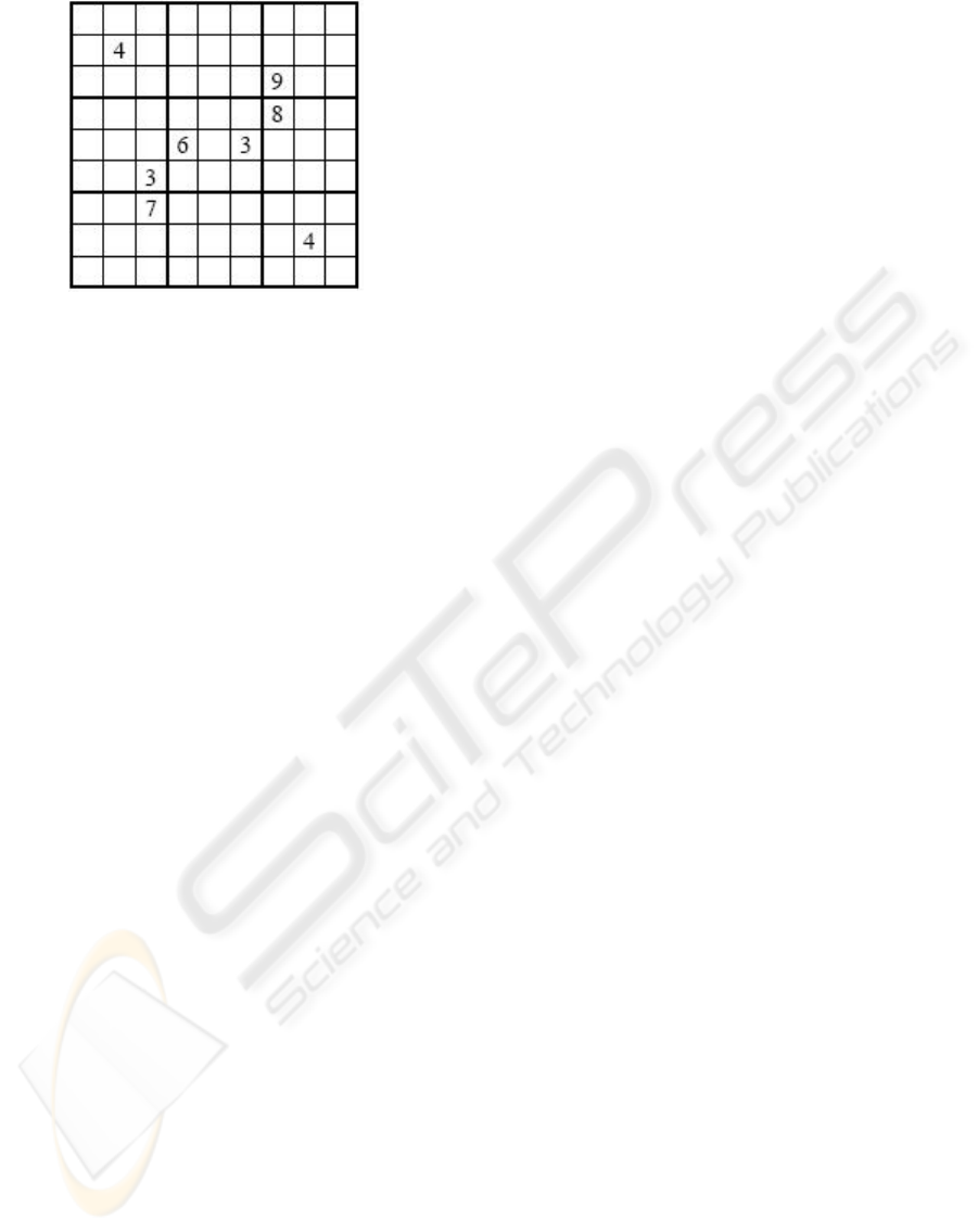
Figure 1: A Quasi-Magic Sudoku Grid (Forbes, 2007b).
(Jones et al., 2007). This is calculated as
3
∏
i=1
3
∏
j=1
n
i j
! (1)
where n
i j
is the number of unassigned cells in the
mini-grid at band i (i = 1, . . . , 3), stack j ( j = 1, . . . , 3).
For the example Sudoku grid shown in Figure 1, with
8 givens, this number is 8! × 9! × 8! × 8! × 7! × 8! ×
8! × 9! × 8! ≈ 2.851 × 10
42
.
4 THE SOLVER
The Quasi-Magic Sudoku puzzle is formulated here
as a state-based problem, requiring definitions for a
cell, a grid of such cells (the state), the means of mod-
ifying the state and pruning conditions to reduce the
size of the search space. This section describes these
components, explaining how the pruning conditions
of Section 3 are incorporated. The use of a heuristic,
that of ordering the cells to be filled according to how
many valid placements of values there currently are
for each cell, is also described. This encourages more
rapid reduction of the search space.
4.1 Definition of a State
A cell is defined in two parts:
• a flag vector, denoting which values may currently
still be assigned to that cell - the candidate values;
• a ‘just fixed’ flag, denoting that the content value
of the cell has recently been fixed.
Initially, each cell has 9 candidate values, and its
value has not been fixed. The flag vector indicates
the candidate values through the use of 9 consecu-
tive bits - each bit representing a different value. Ini-
tially, all bits are set to 1. A value may be designated
as not assignable to a cell (for example because the
value has already been assigned to another cell in the
same row, column or mini-grid) by setting the bit to
zero. This process of masking bits removes a candi-
date value from the cell. Once a value has been as-
signed to a cell, the ‘just fixed’ flag of the cell is set
as a cue to consider the consequences of assignment.
We note that this approach mimics a technique that
may be employed by human solvers, in marking up
candidate numerals in the non-fixed cells.
A puzzle state is simply a grid of 81 cells, and is
used to record the cells currently fixed and the candi-
date values for all remaining non-fixed cells.
Another important consideration in the state def-
inition is the formation of valid rows, columns and
diagonals in the mini-grids of a Quasi-Magic Sudoku
grid. A sequence of three values in a row, column or
diagonal of a mini-grid will be referred to as a triple; a
triple that conforms to the quasi-magic sum constraint
15 ± ∆ (∆ = 2) will be referred to as a qm-triple.
4.2 Search Technique
The search approach employs a backtracking al-
gorithm to perform a depth-first search (Rich and
Knight, 1991) of a puzzle search space. At each
stage, it attempts to assign a value to the next cell
to be considered, by selecting the numerically lowest
of the remaining candidate values for that cell. This
assignment may have far-reaching consequences for
the grid, and it is necessary to propagate these conse-
quences throughout the grid (Section 4.3).
The quasi-magic pruning rules are split into two
groups, one of which is implemented whenever a cell
is assigned a value (Section 4.3); the other is imple-
mented in a pre-processing stage (Section 4.4). Two
approaches are taken to ordering the assignment of
values to cells (Section 4.5). Finally, the backtracking
algorithm itself is detailed in Section 4.6.
4.3 Propagating the Consequences of a
Cell Assignment
During the process of solving a puzzle, cells in the
grid will be fixed to have a specific value. This will
happen either directly, as an attempted step in the so-
lution of a puzzle, or indirectly, as a result of the flag
vector of a cell being reduced to a single candidate so-
lution. On each occasion that an assignment is made,
it is necessary to propagate the consequences of the
assignment throughout the grid. This involves firstly
removing the assigned value as a candidate from all
other cells in the same row, the same column, and the
same mini-grid. This is achieved by masking the ap-
propriate bit from the flag vectors of all such asso-
A KNOWLEDGE-RICH APPROACH TO THE RAPID ENUMERATION OF QUASI-MAGIC SUDOKU SEARCH
SPACES
249

Algorithm 1 : Propagation Algorithm.
Grid is the matrix of cells
Current cell is the cell to which an assignment has
been made
Current value is the value assigned to Current cell
Valid grid is a Boolean flag, initially set to TRUE
for each cell, Cell c, in the same row, column, or
mini-grid as Current cell do
Mask Current value from Cell c
if Cell c is reduced to now having a single can-
didate value then
set ‘just fixed’ flag of cell
end if
end for
if Grid contains a cell having no candidate values
then
set Valid grid to FALSE and terminate PROPA-
GATION
end if
for each row, column and diagonal in which Cur-
rent cell forms a triple do
if the triple is completed, but is not a qm-triple
then
set Valid grid to FALSE and terminate PROP-
AGATION
else if the triple has one unassigned cell then
Check the flag vector of the unassigned cell
for candidate values
if the triple can not become a qm-triple then
set Valid grid to FALSE and terminate
PROPAGATION
end if
end if
end for
for each cell, Cell c, in Grid having ‘just fixed’ flag
set do
Clear ‘just fixed’ flag of cell
Call PROPAGATION recursively
for each rule, Rule r, of the pruning rules 3 to 10
that can apply to Cell c do
if Rule
r is violated by Cell c then
set Valid grid to FALSE and terminate
PROPAGATION
end if
end for
end for
ciated cells. However, this process may have other
consequences for the grid:
• an updated cell may be reduced to having just one
remaining candidate;
• an updated cell may be reduced to having no re-
maining candidates;
• a qm-triple constraint may be violated;
• a quasi-magic pruning rule may be violated.
The assignment of a value to a cell is indicated
by the ‘just fixed’ flag of the cell becoming set, trig-
gering a call to the Propagation Algorithm outlined
above. This algorithm returns a Boolean value indi-
cating whether an assignment is valid, but it also al-
ters the current grid, restricting flag vectors and fixing
cells that have indirectly been limited to a single can-
didate value. A grid is rejected if any cell is reduced to
having no remaining candidate values, as this makes
the grid impossible to complete.
A grid is rejected if a completed triple is definitely
not a qm-triple. It is also rejected if a triple having one
non-fixed cell can not become a qm-triple given its
remaining candidate values. (Note that the algorithm
does not check whether a triple in which two cells
are currently not fixed may still become a qm-triple;
it was deemed that this check would seldom result in
rejection and would cost more in processing time to
execute than would be saved in search space pruning.)
For every cell now having the ‘just fixed’ flag
set, the algorithm is called recursively to propagate
its consequences. The ‘just fixed’ flag of the current
cell is cleared to avoid unnecessary recursion. Any
pruning rule that might be violated by the fixed cell
is checked. (Recall from Section 3 that the pruning
rules relate to specific positions in a mini-grid and so,
for example, a cell assignment at the corner of a mini-
grid could not possibly violate rule 6.)
4.4 Pre-processing of the Grid
Algorithm 2 : Pre-processing Algorithm.
for each given value do
call PROPAGATION
end for
Apply pruning rules 1 and 2
An empty grid is transformed to a puzzle state by
the addition of the given values. The placement of
a given value is treated simply as the assignment of
a cell to a specific value, masking all other candidate
values from the cell’s flag vector. The setting of the
cell’s ‘just fixed’ flag causes the Propagation Algo-
rithm to be called, determining the consequences of
the assignment. At this stage, it is also useful to apply
quasi-magic pruning rules 1 and 2, restricting the can-
didate values of the mini-grid centres and the avail-
able positions for the valid placement of the value 5.
The Pre-processing Algorithm, to prune the search
space to take into account the givens and first two
pruning rules, is as above.
ICAART 2009 - International Conference on Agents and Artificial Intelligence
250

4.5 Cell Ordering
A further dynamic pruning of the search space is im-
plemented through an ordering of the assignments to
cells. Rather than considering cells in some consec-
utive order in terms of their physical position in the
grid, they could instead be ordered according to how
few remaining candidate values they possess. The
main tool in dynamically pruning the search space
is the propagation of the consequences of assigning
a value to a cell throughout the associated row, col-
umn and mini-grid; this effectively prunes up to 20
fruitless branches. The cell ordering heuristic follows
the belief that by favouring assignment to cells hav-
ing fewest candidates, this process of pruning through
propagation will be enacted more rapidly. It is impor-
tant to note that this heuristic does not cause useful
portions of the search space to be overlooked.
A comparison of solution times is made in Section
5 between row-by-row ordering (selecting all cells
across a row before moving to the next neighbouring
row) and this fewest-candidate ordering. We note that
this cell ordering would also seem to mimic a typical
solution strategy employed in manual solution - that
of scanning the grid for cells in which candidate val-
ues may be eliminated.
4.6 Backtracking Algorithm
The algorithm performs a full enumeration of that part
of the search space that has not been pruned by the
Propagation Algorithm. This means that the search
procedure does not stop when the solution is found,
but continues until all possible remaining states have
been enumerated, confirming the uniqueness of solu-
tion (where appropriate). This is particularly useful
for the intended application of Quasi-Magic Sudoku
to the construction of erasure codes, for which it is
important to be certain that every grid can be recon-
structed from a partial grid in a reasonable length of
time. Hence the assurance that the resulting pruned
search space can rapidly be fully enumerated from a
partial grid of givens would be a useful first step in
establishing the general applicability of Quasi-Magic
Sudoku. The backtracking algorithm is as below.
The iteration count, a global counter for the num-
ber of attempted direct assignments of values to cells,
is used in Section 5 as one measure of algorithm per-
formance. Note that many cells are fixed indirectly,
as a result of the propagation algorithm. This will be-
come clearer in Section 5. The recursive call takes the
search process further down the current branch of the
search space (Rich and Knight, 1991).
Algorithm 3 : Backtracking Algorithm.
Grid is the matrix of cells
Set Current cell to be the next cell to be fixed (ac-
cording either to row-by-row or fewest-candidate
ordering)
if there are no cells then
note Grid as a solution
else
for each candidate value in the flag vector of
Current cell do
Increment the Iteration Count
Current value is the next candidate value of
Current cell
Create a local copy of the grid,
Grid local copy.
In Grid local copy, assign Current cell the
Current value
Call PROPAGATION
Call BACKTRACKING (recursively) with the
modified Grid local copy
end for
end if
5 RESULTS AND EVALUATION
To demonstrate the speed of the full enumeration of
the search space, a relatively low-specification ma-
chine was chosen for all tests - an HP-Compaq tc1100
Pentium-m 1GHz portable tablet PC, with 1.5GB
RAM. The algorithm was implemented in Sun’s Java
1.6.0 5 run-time environment; the code was run in de-
bug mode, and was not optimised in any way (such as
obfuscation to reduce variable name lengths).
Quasi-Magic Sudoku puzzles are not commonly
published, but a test set of 180 puzzles was assembled
from (Forbes, 2007a) and (Forbes, 2007b). In Su-
doku, the relationship between the number of givens
and puzzle complexity (measured in accordance with
how long human solvers take to solve them) is not
simple (Jones et al., 2007). As it might reasonably be
assumed that this holds also for Quasi-Magic Sudoku
puzzles, and as no consistent measure of puzzle com-
plexity was generally available for the puzzles of the
test set, the results are categorised purely in terms of
the numbers of givens. The largest number of givens
was 18, and the smallest 4. (It is worth recalling that
although for Sudoku, the smallest reported number of
givens is 17 (Royle, 2006), the additional quasi-magic
rules enable uniqueness of solution to be guaranteed
with far fewer givens.)
The authors know of no published work on the
automated solution of Quasi-Magic Sudoku puzzles.
A comparison is presented here of four different ap-
A KNOWLEDGE-RICH APPROACH TO THE RAPID ENUMERATION OF QUASI-MAGIC SUDOKU SEARCH
SPACES
251
Table 1: Summary of results for all puzzles by solution method: numbers of iterations and processing times (s) for full
enumeration of non-pruned search space.
No q-m No q-m With q-m With q-m
pruning rules pruning rules pruning rules pruning rules
row-by-row fewest-candidate row-by-row fewest-candidate
average iterations 71097 30889 24457 2055
maximum iterations 755373 1172274 214060 51594
minimum iterations 105 28 103 4
median iterations 15963 1608 4658 226
average time (s) 1.6924 0.7984 0.5927 0.0519
maximum time (s) 19.0022 30.6051 5.4582 1.2986
average time per
iteration (ms) 0.0238 0.0258 0.0242 0.0252
proaches to solving the problem, to analyse the use-
fulness of the quasi-magic pruning rules of Section 3
and the fewest-candidate ordering of cells proposed in
Section 4.5. The latter is compared with row-by-row
ordering. All approaches employ checking of whether
mini-grid triples are qm-triples (Section 4.1). The ap-
proaches are:
• no quasi-magic pruning rules, row-by-row cell or-
dering;
• no quasi-magic pruning rules, fewest-candidate
cell ordering;
• quasi-magic pruning rules, row-by-row cell order-
ing;
• quasi-magic pruning rules, fewest-candidate cell
ordering.
Runs of the algorithm are analysed here as to the
time taken (in seconds, to 4 decimal places), and the
number of iterations (to the nearest integer) which had
to be performed to complete each puzzle (as defined
in Section 4.5). As the backtracking algorithm per-
forms a full enumeration of that part of the search
space that has not been pruned by the pruning con-
ditions and qm-triple checks, the results presented
here are not skewed by puzzles for which the solution
is ‘conveniently’ positioned within the search space.
The results obtained are therefore an accurate mea-
sure of the relative sizes of the non-pruned search
spaces of the puzzles, and not just a measure of how
rapidly a solution may be found.
Table 1 shows a summary of the results for all puz-
zles in the test set, arranged by solution method. This
table shows a consistent drop in average iterations and
average time across methods, but examination of the
other results indicates that the cell ordering has the
most significant impact on reducing the number of
iterations. The addition of the quasi-magic pruning
rules is delivered at a smaller overhead in processing
time than the fewest-candidate cell ordering, but the
average and median iterations would support the view
that both modifications are worth implementing. The
changes in the average time per iteration (measured in
milliseconds) are clearly slight. For some puzzles re-
quiring larger numbers of iterations to enumerate the
search space, the use of fewest-candidate cell order-
ing actually increases the number of iterations, but the
number is reduced for the majority of puzzles. This
behaviour is not observed when the quasi-magic prun-
ing rules are also added.
Through the additional analysis of the breakdown
of results into categories of numbers of givens (Ta-
ble 2), it is clear that the combination of quasi-magic
pruning rules and fewest-candidate cell ordering is by
far the best method. The number of puzzles in each
category of number of givens is shown in parenthe-
sis. Irrespective of whether there is an entirely uni-
form correlation between the number of givens and
the ease with which a puzzle may be solved by hand
(Jones et al., 2007), it seems clear that a strong cor-
relation exists with the speed with which this solver
enumerates the non-pruned search spaces of Quasi-
Magic Sudoku puzzles. The processing overhead of
the quasi-magic pruning rules starts to become appar-
ent on the fastest enumerating puzzles, but not enor-
mously so; the addition of fewest-candidate cell or-
dering seems to overcome this.
Table 3 shows more detailed results, categorised
by the number of givens, for the most successful
method - quasi-magic pruning rules with fewest-
candidate cell ordering. The worst case in the test
set, a puzzle having 6 givens, took 51,594 iterations
(which corresponded to 1.2986 seconds) to fully enu-
merate the non-pruned search space. The overwhelm-
ing majority of the puzzles in the test set required less
than 0.1 seconds. The average time per iteration is re-
markably constant for all but those puzzles requiring
very few iterations. For the declared application, it is
sufficient to know that the non-pruned search spaces
ICAART 2009 - International Conference on Agents and Artificial Intelligence
252
Table 2: Average time (s) for all solution methods, by number of givens.
No q-m No q-m With q-m With q-m
pruning rules pruning rules pruning rules pruning rules
row-by-row fewest-candidate row-by-row fewest-candidate
<7 (12) 7.8336 3.7024 2.5663 0.4451
7-8 (49) 3.3064 1.8388 1.1547 0.0593
9-10 (35) 1.1229 0.1879 0.4348 0.0205
11-12 (45) 0.1706 0.0485 0.0710 0.0057
13-14 (29) 0.0511 0.0130 0.0274 0.0030
>14 (10) 0.0159 0.0043 0.0111 0.0022
Table 3: Iterations and average time per iteration of the method employing quasi-magic pruning rules and fewest-candidate
cell ordering, by number of givens.
number of average maximum median average time per
Givens iterations iterations iterations iteration (ms)
<7 (12) 17,984 51,594 13,051 0.0248
7-8 (49) 2,351 21,586 1,119 0.0252
9-10 (35) 796 7,006 300 0.0258
11-12 (45) 186 933 140 0.0309
13-14 (29) 80 303 52 0.0377
>14 (10) 41 108 30 0.0529
of all puzzles can rapidly be fully enumerated.
The algorithm described in Section 4 is very effi-
cient. Due to the compact representation of the grid
and the early rejection of unpromising states, the im-
plementation of the algorithm has very low memory
requirements; it requires less than 100KB of work-
ing RAM to run. (The updating of the flag vectors of
cells, through bitmasking, is greatly faster than, for
example, the indexing of candidate value information
stored as elements in an array.) This approach is also
scalable, enabling the prospect of similar acceptable
results being achievable for larger Quasi-Magic Su-
doku puzzles, for example of size 64.
6 CONCLUSIONS
This paper demonstrates that domain information for
Quasi-Magic Sudoku puzzles, for the case ∆ = 2, may
be used to reliably and rapidly reconstruct a grid,
from a small set of given values. The knowledge-rich
quasi-magic pruning rules and the proposed cell or-
dering both contribute to a massive reduction in the
size of the search space that needs to be enumerated,
both to determine a solution and, importantly here, to
be certain of the uniqueness of that solution.
In a general sense, the above findings establish
the applicability of Quasi-Magic Sudoku for the con-
struction of erasure correction codes. This is an im-
portant result, given that Sudoku codes have already
been established as being of interest (Soedarmandji
and McEliece, 2007), and Quasi-Magic Sudoku car-
ries the prospect of grid reconstruction (and hence
message reconstruction) from a smaller set of initial
given values. However, to prove the usefulness of
Quasi-Magic Sudoku in erasure correction, it is nec-
essary also to consider reconstruction from a set of
values which may not correspond well to the minimal
set of independent givens of a particular grid.
As additional further work, we propose the exami-
nation of other cases of ∆, to determine corresponding
domain-rich cell value interrelationships and associ-
ated pruning rules. Other cell orderings, derived from
an understanding of the puzzle, might yield further re-
ductions in the search space. The determination of the
numbers of valid grids for other cases of ∆ would also
be of mathematical interest. The examination of puz-
zles of larger sizes might also be useful within cod-
ing theory and other applications. Lastly, it is pro-
posed that an analysis is performed of how frequently
each of the quasi-magic pruning rules of Section 3 is
employed in pruning the search space, and which are
most effective for the least cost in processing time.
REFERENCES
Bartlett, A. and Langville, A. (2006). An inte-
ger programming model for the sudoku problem.
Preprint available at http://www.cofc.edu/ langvil-
lea/Sudoku/sudoku2.pdf. Cited 1 Jun 2008.
A KNOWLEDGE-RICH APPROACH TO THE RAPID ENUMERATION OF QUASI-MAGIC SUDOKU SEARCH
SPACES
253

Felgenhauer, B. and Jarvis, F. (2006). Mathematics of su-
doku I. Mathematical Spectrum, 39:15–22.
Forbes, T. (2007a). Quasi-magic sudoku puzzles. M500,
215:1–10.
Forbes, T. (2007b). Sudoku puzzles.
http://anthony.d.forbes.googlepages.com/sudoku.htm
Cited 1 June 2008.
Gomes, C. and Shmoys, D. (2002). The promise of lp to
boost cp techniques for combinatorial problems. Pro-
ceedings of the Fourth International Workshop on In-
tegration of AI and OR techniques in Constraint Pro-
gramming for Combinatorial Optimisation Problems,
pages 291–305. France.
Jones, S. K., Perkins, S., and Roach, P. A. (2008). Quasi-
magic sudoku. in prep.
Jones, S. K., Roach, P. A., and Perkins, S. (2007). Construc-
tion of heuristics for a search-based approach to solv-
ing sudoku. Research and Development in Intelligent
Systems XXIV: Proceedings of AI-2007, the Twenty-
seventh SGAI International Conference on Artificial
Intelligence.
McWilliams, F. and Sloane, N. (1977). The Theory of Error-
Correcting Codes. Elsevier: Amsterdam.
Moraglio, A. and Togelius, J. (2007). Geometric particle
swarm optimization for the sudoku puzzle. Gecco-
Conference Conf 9, 1:118–125.
Moraglio, A., Togelius, J., and Lucas, S. (2006). Product
geometric crossover for the sudoku puzzle. Proceed-
ings of the IEEE Congress on Evolutionary Computa-
tion, pages 470–476.
Rich, E. and Knight, K. (1991). Artificial Intelligence.
McGraw-Hill, 2 edition. Singapore.
Royle, G. (2006). Minimum sudoku. Internal Report,
http://people.csse.uwa.edu.au/gordon/sudokumin.php.
Cited 1 Jun 2008.
Simonis, H. (2005). Sudoku as a constraint problem.
Modelling and Reformulating Constraint Satisfaction
Problems, pages 13–27.
Soedarmandji, E. and McEliece, R. J. (2007). Iterative de-
coding for sudoku and latin sqaure codes. Forty-Fifth
Annual Allerton Conference, pages 488–494.
ICAART 2009 - International Conference on Agents and Artificial Intelligence
254
