
FROM REACTIVE MULTI-AGENTS MODELS
TO CELLULAR AUTOMATA
Illustration on a Diffusion-Limited Aggregation Model
Antoine Spicher
1
, Nazim Fat`es
2
and Olivier Simonin
2
1
LACL, Universit´e Paris 12, 61 avenue du G´en´eral de Gaulle, 94010 Cr´eteil, France
2
LORIA - INRIA Nancy Grand Est, Campus Scientifique, 54506 Vandœuvre-l`es-Nancy, France
Keywords:
Reactive multi-agent systems, Cellular automata, Influence-reaction model, Diffusion-limited aggregation.
Abstract:
This paper deals with the synchronous implementation of situated Multi-Agent Systems (MAS) in order to
have no execution bias and to allow their programming on massively parallel computing devices. For this pur-
pose we investigate the translation of discrete MAS into Cellular Automata (CA). Contrarily to the sequential
scheduling generally used in MAS simulations, CA are a model for massively parallel computing where the
updating of the components is synchronous. However, CA expressiveness is limited and not always adapted
to build models where independent entities move and act on neighbor cells. After illustrating these issues on
a simple example, we propose a generic method to translate a discrete MAS into a CA, called a transactional
CA. Our approach consists in using the influence-reaction model to perform this translation.
1 INTRODUCTION
Multi-agents systems (MAS) are widely used for
modeling systems where autonomous entities, the
agents, move in a virtual space, the environment, and
act on it. Numerous simulators and platforms have
been developed to simulate such systems. However,
in these tools, the updating of the agents is often left
as a hidden procedure, on which the user has no con-
trol. The most common updating procedure is the
sequential procedure: agents are updated one after
the other with an order fixed in advance (often ran-
domly). It is a well-knownproblem that such schedul-
ing is a potential source of biases, i.e., it may intro-
duce causalities that were not designed by the user but
come only from the simulating tool. By contrast, Cel-
lular automata (CA) are a well-known model of mas-
sively parallel computing devices where the updating
of the components is synchronous: all the cells are up-
dated at once without any priority between them. The
advantage of using the CA formalism is simplicity:
it involves static homogeneous computing units that
are regularly arranged in space. The drawback of ex-
pressing a model with cellular automata appears when
one needs to build models with pseudo-independent
entities that may move and act on neighbor cells. In-
deed, in CA, a cell cannot directly change the state of
its neighbor cells, whereas such an ability is usually
required to express a MAS model. This paper investi-
gates the translation of discrete MAS models into CA,
which is illustrated on a simple example. The inter-
est is twofold: (1) to have a synchronous execution of
agents and thus to reduce bias due to the update, and
(2) to ease the programming of MAS on massively
parallel computing devices such as FPGAs or GPUs.
The purpose of our research is to find a method to
translate ”the language of multi-agents” into ”the lan-
guage of cellular automata”. In this article, we pro-
pose to take advantage of both contexts, the high ex-
pressiveness of a MAS specification and the simplic-
ity of a CA implementation. We aim at developing
a framework where MAS, that are simply described
through the separate specifications of the local agent
behaviors and the environment dynamics, are auto-
matically translated as a uniform transition function
of a CA.
This article is organized as follows: In Section 2,
we discuss the relations between CA and MAS ap-
proaches. Section 3 introduces the concept of trans-
actional CA, starting from the study of a paradigmatic
example of a MAS model, namely the Diffusion-
Limited Aggregation model. Section 4 proposes the
422
Spicher A., Fatès N. and Simonin O. (2009).
FROM REACTIVE MULTI-AGENTS MODELS TO CELLULAR AUTOMATA - Illustration on a Diffusion-Limited Aggregation Model.
In Proceedings of the International Conference on Agents and Artificial Intelligence, pages 422-429
DOI: 10.5220/0001660404220429
Copyright
c
SciTePress

first step of a formal description allowing the generic
coding of a reactive MAS model into a transactional
CA. We finally conclude with discussions on related
and future works.
2 MAS VERSUS CA
At first sight, the two formalisms look very similar
and are often confused. One may find several works
where the names “cellular automata” and “multi-
agent systems” are used without distinction. This
is easily understandable since CA are often used to
model the environment of a MAS, and, reciprocally,
one may see a CA as a particular kind of MAS where
agents do not move.
We now clarify the differences between CA and
MAS in the context of our research. We compare
them at two levels: (1) the modeling level: What in
a model makes CA or MAS more suitable to express
it? (2) the simulation level: How intuitive is the im-
plementation of CA and MAS?
MAS and CA, as Modeling Tools. In their def-
inition, CA are uniform objects: there is a unique
neighborhood shape for each cell and a unique tran-
sition function. As a consequence, CA are fitted to
model phenomena that involve homogeneous spaces;
CA have been used for example to model physical
systems (Chopard and Droz, 2005), biological sys-
tems (Deutsch and Dormann, 2005), spatially em-
bedded computations (Adamatzky, 2001), etc. Note
that it is always possible to take into account inhomo-
geneities, for example by encoding the heterogeneity
in the cell states, but this is generally not straightfor-
ward to do so.
MAS are preferred for expressing an heteroge-
neous population of entities. They necessitate to
make a distinction between the agents’ behaviors and
the environment where they are embedded (Ferber,
1999). This distinction allows to focus on the spec-
ification of particular and localized events, namely
the agents actions. They offer a methodology for
designing systems, at the level of algorithms, pro-
gramming languages, hardware, etc. Examples of
MAS applications range from the simulation of nat-
ural systems, from ants (Resnick, 1994) to human be-
haviors (Regelous, 2004), to the design of massively
distributed software and algorithms like web-services,
peer-to-peer technologies, etc. Nevertheless, we must
note that contrarily to CA, no universal definition of
MAS has been accepted so far. From the modeling
point of view, translating MAS in the cellular au-
tomata formalism has (at least) the advantage of fix-
ing the mathematical expression of the model and re-
moving ambiguities of formulation.
MAS and CA, as Simulation Tools. The key char-
acteristic of complex systems is the difficulty, if not
the impossibility, of inferring their global behavior
from the local specification of the interactions. Few
mathematical tools are available to predict the evolu-
tion of complex systems, more especially those which
involve self-organization. This gives to simulation a
central role to find the mechanisms that explain how
complexity emerges from simple local interactions.
We thus have to pay attention to the quality of sim-
ulations and to detect ambiguities that may be hidden
in the way they are implemented.
The agent-based programming style is somehow
intuitive and natural as the programmer takes the
point of view of the agent. There is a form of an-
thropomorphism that makes MAS programming par-
ticularly attractive. Nevertheless, we emphasize that
once all the agents behaviors are individually speci-
fied, there are still many ways to make the agents in-
teract and play together in the environment. The im-
plementation of such systems raises many questions,
like assessing the importance of the synchronicity in
simulations: are the agents updated all together or
one after the other? The design of spatially-extended
computing devices will require to imagine a new type
of computer science, where the computations do not
necessarily rely on the existence of a synchronization
between the components.
By contrast with MAS, CA lead to shift the pro-
grammer’s point of view from the “eyes” of the agents
to their environment. The benefits of this shifting ef-
fort are twofold: (1) the CA formalism forces the pro-
grammer to solve conflicts between concurrent agents
actions at the elementary level of the cell and for-
bids the use of any global procedure. (2) As a conse-
quence, the implementation on massively distributed
devices is easy. Indeed, CA provide the program-
mer a cell-centered programming style where the set
of cells represents computing units that are regularly
organized. Recent works have shown that it is pos-
sible to have a good efficiency by using parallel ar-
chitecture to run CA simulations for GPU and for
FPGA, e.g. (Halbach and Hoffmann, 2004). In other
words, CA provide an easy-to-implement framework,
but expressing the local rule necessitates a method to
“blend” the different components of a complex sys-
tem.
FROM REACTIVE MULTI-AGENTS MODELS TO CELLULAR AUTOMATA - Illustration on a Diffusion-Limited
Aggregation Model
423

3 THE DLA EXAMPLE AS A
STARTING POINT
In this section, we introduce our approach through the
translation of a simple MAS model into an original
kind of CA, called transactional CA. For this purpose,
we focus on the CA encoding of a diffusion-limited
aggregation (DLA) system. This example presents a
good trade-off between the simplicity of description
and the richness of problems risen by this coding.
The DLA model was introduced to study phys-
ical processes where diffusing particles, following
a Brownian motion, aggregate (Witten and Sanders,
1981): for instance, zinc ions aggregate onto elec-
trodes in an electrolytic solution. This process leads
to interesting self-organized dendritic fractal struc-
tures. Different models of DLA have been proposed;
we consider in this article that particles stick together
forever and that there is no aggregate formation be-
tween two mobile particles.
3.1 MAS Specification of the DLA
The MAS specification of the DLA model describes
separately the agents and the environment where they
evolve:
The Environment is a 2D finite and toric square grid
composed of elements called patches. The exclu-
sion principle holds: i.e., there cannot be more
than one agent on each patch of the grid.
The Population of Agents, denoted by A , is com-
posed of the particles. Each particle a of A is lo-
calized on a cell ρ
a
of the environmentand is char-
acterized by a state σ
a
: a particle is either Fixed
or Mobile.
The initial configuration of the system is composed of
a population of Mobile particles and some Fixed par-
ticles called the seeds. The expected behavior is the
aggregation of the Mobile particles to build dendrites
from the seeds.
We propose to formulate the agent dynamics using
the usual perception-decision-action cycle (Brooks,
1990). We first describe the perception and action
abilities of an agent. The perception consists of two
functions:
• Γ
1
returns true if the agent perceives a Fixed
neighbor particle, and false otherwise;
• Γ
2
computes the set of directions that lead to
empty neighbor patches.
The neighborhood referred in these perceptions cor-
responds to the four closest positions of ρ
a
following
North, South, East and West directions. The set of
actions is:
• Diffuse(d): move following direction d;
• Aggregate: change to the Fixed state;
• Stay: do nothing
Let U (S) denote the operation of selecting one ele-
ment in a finite set S with uniform probability, the de-
cision process returns an action as a function of the
agent perceptions:
if Γ
1
then Aggregate
else if Γ
2
6=
/
0 then Diffuse(U (Γ
2
))
else Stay
(1)
3.2 CA Expression of the DLA Model
We now reach the core of the problem. We first dis-
cuss about implementing the agent motion within a
synchronous computational model. We then propose
our solution, called transactional CA, and we finally
illustrate it on the DLA example.
The Synchrony Paradox. In the MAS style of pro-
gramming, emphasis is put on the agents local behav-
iors. Classically, to avoid collisions between mobile
particles, they are introduced one after the other, or
in some cases, are introduced simultaneously but up-
dated one after the other using a scheduler. However,
two objections can be raised:
1. The implementation of this sequential updating
on a massively distributed computing device is
not impossible, but it requires the introduction of
complex procedures to synchronize the different
schedulers.
2. The use of a scheduler introduces an external form
of causality that was not specified in the original
DLA formulation. This may induce a bias in the
formation of dendritic patterns, especially when
the density of mobile particles is high.
By contrast, the framework of CA demands an early
resolution of the conflicts created by simultaneous
moves to a given patch. To achieve that, we propose
to establish a dialog between cells.
Transactional CA. A particle move requires a
source cell (that contains a particle at time t) and a
target cell (that will contain the particle at time t + 1).
We propose to elaborate a three-step transactional
process where cells negotiate their requirements:
1. Request: source cells express their needs to their
neighbors.
2. Approval-rejection: target cells accept or not their
neighbors requirements; this decision is done with
ICAART 2009 - International Conference on Agents and Artificial Intelligence
424
Target
time
Request Approval Transaction
Source
otherwise
otherwise
exactly one request
otherwise
from direction d
′
M
1
S
F
0
M
0
M
0
E
0
E
0
F
0
E
1
E
2
F
1
F
2
F
1
A F
2
A
M
2
S
R
2
(d
′
)
M
2
D(d)M
1
D(d)
Γ
1
d ∈ Γ
2
q
d
= R
2
(−d)
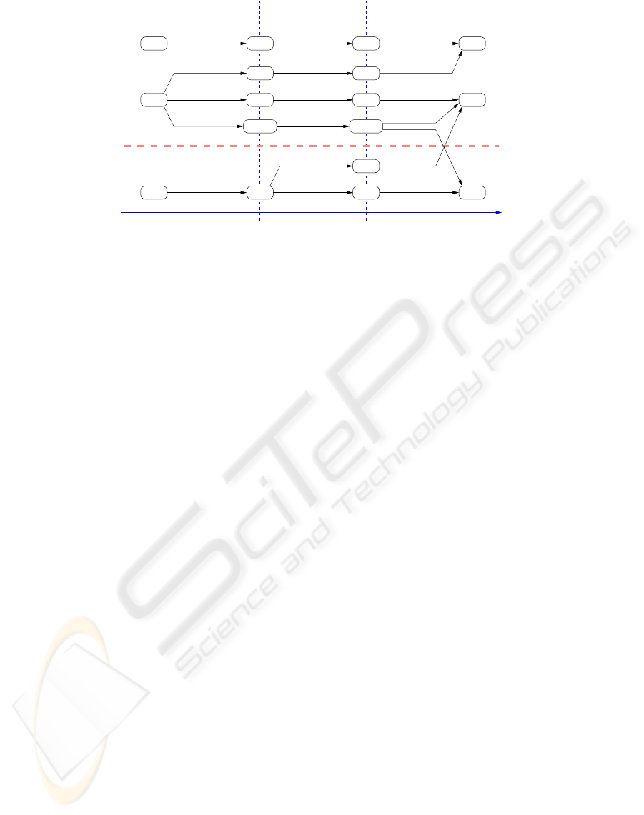
Figure 1: DLA local evolution rule within a transactional CA. This graph shows the local evolution of a cell from a state to
another depending on its neighborhood state. Explanations are given in the text.
respect to an exclusion principle policy (for exam-
ple, an empty cell is an available target if and only
if there is exactly one particle requesting to move
to this cell).
3. Transaction: sources and targets separately
evolve.
DLA Transaction Model. Figure 1 shows with a
graph the local transition function of a transactional
CA capturing the agent-based specification of the
DLA given in section 3.1. On this graph, nodes rep-
resent the different states of the CA (states E
0
, F
0
and
M
0
are given twice to clarify the figure) and the ar-
rows specify transitions between states. States are dis-
tributed
• vertically, to segregate the behaviors of sources
and targets, and
• horizontally, to distinguish the three steps of a
transactional CA.
At the beginning, the cells are either empty or contain
a particle which is either fixed or mobile: three states
are used E
0
, F
0
and M
0
.
• The request transition consists in deciding an ac-
tion for each M
0
cell: depending on the percep-
tions, a mobile particle either aggregates (state
F
1
A), or requests diffusion following a direction
d (state M
1
D(d)), or stays at the same position
(state M
1
S).
• During the approval step, empty cells E
1
de-
cide, by reading their neighbors requirements, if
they remain empty (state E
2
) or become recep-
tors of particles moving from a direction d
′
(state
R
2
(d
′
)).
• Finally, the transaction is computed: receptors be-
come particles, mobile particles that target a re-
ceptor (i.e., when the state q
d
of the pointed cell
is R
2
(−d), where −d denotes the direction op-
posite to d), become empty, and aggregating par-
ticles become fixed. Other cells remain in their
initial state.
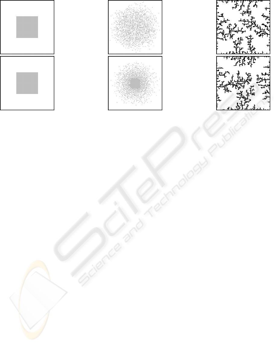
Figure 2 presents simulations of the previous de-
scribed DLA model in two simulations frameworks.
On the first line, simulations were obtained using a
classical sequential framework based on a scheduler,
on the second line, we display simulations of our syn-
chronous transactional CA. The same initial config-
uration, given on the left column, was used on both
platforms. It consists of a 100x100 grid where seeds
are localized on the boundaries and where mobile par-
ticles are gathered in a 40x40 central square. Both
systems exhibit the same qualitative behavior, as seen
on the right column of Figure 2. However, further
studies on the dendrites distribution or on the mean
time required to reach a fixed point would be needed
to assess the differences between the two approaches.
To compare the time scales of the two systems, we
define a simulation time step as: (a) the three sub-
steps of the transactional CA and (b) the update of
all the agents in the sequential framework. We ob-
serve that the dissolution of the initial square is slower
in the synchronous CA than it is in the MAS model
with a sequential updating (see the middle column of
Figure 2). A simple explanation of this phenomenon
is that an asynchronous update allows a particle to
move to a just evacuated patch during a simulation
time step, while the synchronous update forbids this
behavior.
FROM REACTIVE MULTI-AGENTS MODELS TO CELLULAR AUTOMATA - Illustration on a Diffusion-Limited
Aggregation Model
425
t = 0 t = 130 t = ∞
Figure 2: DLA Simulations: from left to right, the initial state, the state after 130 simulation time steps and the fixed point,
with in black the fixed particles and in gray the mobile particles. The first line was obtained using the sequential simulation
tool TurtleKit (Michel et al., 2003), the second was obtained using the CA simulation tool FiatLux (Fat`es, 2008b).
4 TOWARDS A
GENERALIZATION
In this section, we investigate how a generic method
could be developed to automatically translate the
specification of a MAS into the transition function
of a transactional CA. Of course, reducing a MAS
to a CA enforces some restrictions on what can be
described. More especially, in order to respect the
finiteness of CA, we assume that MAS are discrete
and finite systems: i.e., the environment is a discrete
and regular grid where a finite number of agents are
localized on specific parts of this grid (they do not
have continuous coordinates).
Our approach is based on the use of the formal
influence-reaction model (Ferber and Muller, 1996)
to describe a MAS. In fact, the three steps of the
transactional CA are similar to the three steps of
influence-reaction: (1) agents produce influences that
are attempts of actions, (2) influences are combined
to avoid conflicts between the corresponding actions,
and (3) the environment is updated with respect to the
combined influences. In the following, we introduce
the influence-reaction model and we finally give the
first step of a formal description of an automatic trans-
lation of an influence-reactionbased specification into
a transactional CA.
4.1 Influence-Reaction Model
On the opposite of the CA, there is no unique formal
description of MAS models. Nevertheless, there exist
some generic models that focus on specific kinds of
MAS (e.g. logic MAS, communicating MAS, etc.).
For the sake of clarity, we only consider situated
MAS that deal with discrete environmentand reactive
agents. The term “situated MAS” relates to systems
where agents are embedded in a “physical” environ-
ment.
In this context, we focus on the influence-reaction
model that is dedicated to the formal description of
situated MAS, allowing, in particular, the simulation
of simultaneous actions (Ferber and Muller, 1996). In
this model, agents release influences that will induce
reactions of the environment. An influence corre-
sponds to attempting an action. The reaction consists
in combining the different influences in order to real-
ize the corresponding actions. This modeling princi-
ple is inspired by physics where entities react because
some forces act on them. Like forces, influences can
be combined. For instance, an influence may be an
attempt to pull a door. If two agents simultaneously
perform this influence with the same intensity from
the opposite sides of a door, the combination of both
influences vanishes and the resulting action is null.
We assume here that the combination of influences
can be computed locally. In other words, the evalua-
tion of the combination function can be distributed on
each patch of the environment. The dynamics of the
three steps of the influence-reaction model may be de-
scribed as follows:
1. Each agent a of A separately computes, as a func-
tion f
a
of its current state σ
t
a
and of its percep-
tions Γ
a
, its new state σ
t+1
a
and the associated set
ICAART 2009 - International Conference on Agents and Artificial Intelligence
426

of influences I
a
. We denote by I the set of all the
possible influences, Σ
A
the set of the agent states.
2. Let I
ρ
denote all the influences produced by the
agents of A that could affect the patch ρ of the
environment (we denote by P the set of all the en-
vironment patches). Each patch ρ separately com-
putes the set
∏
I
ρ
of combined influences affect-
ing this patch.
3. Finally, for each patch ρ of the environment, the
new state σ
t+1
ρ
of ρ is computed as a function f
E
of the current position state σ
t
ρ
with respect to the
set of influences
∏
I
ρ
. We denote by Σ
E
the set of
the patch states.
Using these notations, the influence-reaction dynam-
ics may be formally summarized by the following two
equations:
hσ
t+1
a
, I
a
i = f
a
(σ
t
a
, Γ
a
) a ∈ A (2)
σ
t+1
ρ
= f
E
(σ
t
ρ
,
∏
I
ρ
) ρ ∈ P (3)
4.2 Generation of a Transactional CA
Formally speaking, a CA is a quadruple (L , Q, N , δ)
where:
• L is the set of cells generally taken as a subset of
Z
dim
, dim is the dimension of the space.
• Q is a finite set of states. Each cell c ∈ L is asso-
ciated with a value q
c
∈ Q.
• Each cell c is associated with a set of cells N (c) ⊂
L called the neighborhood of c. The relation-
ship N expresses the locality of interactions, i.e.,
N (c) is constituted of cells “close” to c.
• The local transition function δ returns a value in
Q that depends on the current state q
c
and on the
states of the cells in the neighborhood N (c).
The generation of a transactional CA consists in
defining these four elements using the different com-
ponents of the MAS specification. For the sake of
simplicity, we restrict ourselves to MAS where:
• the set P corresponds to a 2D regular square grid
(dim = 2);
• an exclusion principle holds, that limits to one the
maximum number of agents on a given patch;
• the set I
a
is always a singleton, that means that an
agent decides to attempt only one action at each
time step. Note that this case is not restrictive,
because any set of influences could be rewritten
as a single influence: if the agent does nothing
(i.e., I
a
=
/
0), we consider that it releases the spe-
cial Skip influence, and if there are more than two
influences (e.g. I
a
= {Depose, Diffuse(d)}), new
symbols are considered in I to capture the corre-
sponding action (e.g. I
a
= Dep oseDiffuse(d));
• the combinationof influences
∏
I
ρ
is always a sin-
gleton. In other words, only one action could af-
fect a position ρ.
As shown on Figure 1, the definition of the transition
function can be divided into three sub-functions δ
0
,
δ
1
and δ
2
corresponding to the three steps of a trans-
actional CA. As a consequence, the set of states Q can
also be partitioned into three subsets Q
0
, Q
1
, Q
2
, de-
pending on the next step of the transactional CA to be
computed.
In the following paragraphs, we detail the key
points of the transactional CA generation. We illus-
trate this translation on the example of the DLA.
Cells and Neighborhood. The set of cells exactly
corresponds to the 2D grid defined by the set of
patches, so L = P . The neighborhood relationship N
is defined in such a way that N (c) gathers the cells
that an agent a, localized on c, may read to compute
its perceptions Γ
a
and its actions I
a
.
As an example, the particles of the DLA model
may remain on the same position, and perceive or
move to the positions following the North, South,
West and East directions. As a consequence, the cor-
responding CA neighborhood relationship N corre-
sponds to the classical von Neumann neighborhood;
for each cell c ∈ L :
N (c) = {c
′
∈ L , ||c− c
′
|| ≤ 1}
where ||c − c
′
|| denotes the graph distance between
two cells.
The Initial States Set Q
0
. The set Q
0
corresponds
to the initial states of a cell before applying the three
steps of the transactional CA. Let c be a cell and ρ its
corresponding patch. The state of c is characterized at
a given time t by
• the environment state σ
t
ρ
at ρ, and
• whether there is an agent a with state σ
t
a
on ρ.
Let
e
Σ
A
denote the set Σ
A
∪ {⊥}, where the symbol ⊥
represents the absence of agent. Then, the state of Q
0
are couples (σ
t
a
, σ
t
ρ
):
(σ
t
a
, σ
t
ρ
) ∈ Q
0
=
e
Σ
A
× Σ
E
For the DLA model, we have Σ
A
= {Mob ile, Fixed}
and Σ
E
=
/
0: the cells of the environment are here pas-
sive and holds no information. So we have:
Q
0
= {Mobile, Fixed, ⊥}
that corresponds to the states M
0
, F
0
and E
0
of Fig-
ure 1.
FROM REACTIVE MULTI-AGENTS MODELS TO CELLULAR AUTOMATA - Illustration on a Diffusion-Limited
Aggregation Model
427

The Request Step and the Set Q
1
. Compared to
the elements of Q
0
, the states composing Q
1
are char-
acterized by an additional information: the influence
chosen with respect to the specification of f
a
(see
Eq. 2). In the case of an ⊥ cell, the particular Skip
influence is used. Considering Equation 2 notations,
the transition function δ
0
is defined by:
δ
0
: Q
0
−→ Q
1
= Q
0
× I
(σ
t
a
, σ
t
ρ
) 7−→
(σ
t
a
, σ
t
ρ
, Skip) if σ
t
a
= ⊥
(σ
t+1
a
, σ
t
ρ
, I
a
) otherwise
Note that the evaluation of the transition function δ
0
depends on the neighborhood state as it requires the
perceptions Γ
a
to compute hσ
t+1
a
, I
a
i using f
a
.
In the DLA model, the set of particle actions is
I = {Diffuse(d), Aggregate, Stay}. If we identify the
neutral Skip action to Stay, the definition of δ
0
, based
on the use of Equation 1, gives:
δ
0
(⊥) = (⊥, Skip)
δ
0
(Fixed) = (Fixed, Skip)
δ
0
(Mobile) =
(Fixed, Aggregate)
(Mobile, Stay) w.r.t. Eq. 1
(Mobile, Diffuse(d))
These transitions correspond to the five arrows of
the “Request” column of the Figure 1. Note that
some states of Q
1
are meaningless (e.g. the state
(Fixed, Diffuse(d)) would correspond to a diffusing
fixed particle).
The Approval Step and the Set Q
2
. During this
step, each cell c, associated with a patch ρ, computes
the set of influences I
ρ
that may affect its state. This
computation is done by reading the third element of
the states of the neighbor cells. Then, the operator
∏
combines these influences into a single influence that
will be taken into account during the transaction step.
As a consequence, states from Q
2
refer to an addi-
tional information: the combined influence
∏
I
ρ
. The
transition δ
1
is then defined by:
δ
1
: Q
1
−→ Q
2
= Q
1
× I
(σ
t+1
a
, σ
t
ρ
, I
a
) 7−→ (σ
t+1
a
, σ
t
ρ
, I
a
,
∏
I
ρ
)
The exclusion principle of the DLA model is specified
by the definition of the operator
∏
. Formally, let ρ be
a patch, I
ρ
the set of actions that affect the state of ρ,
and |S| the cardinal of a finite set S, we have:
δ
1
(⊥, Skip) =
(⊥, Skip, I
ρ
) if |I
ρ
| = 1
(⊥, Skip, Skip) otherwise
δ
1
(σ
a
, I
a
) = (σ
a
, I
a
, Skip)
The state (⊥, Skip, I
ρ
) corresponds to the state R(d
′
)
of Figure 1: this state is only reachable from an empty
patch with exactly one request of move.
The Transaction Step. The final step consists in
computing a new state of Q
0
as a function of a state
of Q
2
:
δ
2
: Q
2
−→ Q
0
The transition δ
2
computes the new state of the patch
ρ and the eventual move of agents from or to ρ. This
computation relies on two pieces of information:
• the influence
∏
I
ρ
that has to be realized, and
• the influence I
a
that is attempted.
As we assume an exclusion principle, we describe
separately the case where the cell is empty and the
case where an agent a is localized on the cell. If the
cell is empty, δ
2
is defined by:
δ
2
(⊥, σ
t
ρ
, I
a
,
∏
I
ρ
) =
(σ
t+1
a
, σ
t+1
ρ
) (1)
(⊥, σ
t+1
ρ
) (2)
where (1) and (2) correspond to two possible cases:
Case (1):
∏
I
ρ
expresses that ρ is a target cell for an
agent a and that this move has to be realized. The
state σ
t+1
a
of this agent comes from the state of the
source cell. On Figure 1, the transition from state
R
2
(d
′
) to state M
0
illustrates this case.
Case (2):
∏
I
ρ
does not allow any agent move to the
patch ρ. On Figure 1, the transition from state E
2
to state E
0
illustrates this case.
In both cases, the state of the environment may be
affected by the influence
∏
I
ρ
. The new σ
t+1
ρ
is com-
puted using Equation 3.
If an agent a is localized on the cell, δ
2
is defined
by:
δ
2
(σ
t+1
a
, σ
t
ρ
, I
a
,
∏
I
ρ
) =
(⊥, σ
t+1
ρ
) (3)
(σ
t+1
a
, σ
t+1
ρ
) (4)
where (3) and (4) correspond to two possible cases:
Case (3): I
a
expresses a move of the agent a from
the patch ρ to another patch ρ
′
where I
a
=
∏
I
ρ
′
(i.e., the action is allowed by
∏
I
ρ
′
). The patch ρ
becomes empty. On Figure 1, the transition from
state M
2
D(d) to state E
0
illustrates this case.
Case (4): I
a
is not allowed by the neighborhood. On
Figure 1, the transition from state M
2
D(d) to state
M
0
illustrates this case.
In both cases, the new σ
t+1
ρ
is computed using Equa-
tion 3.
5 DISCUSSION
The transactional CA we proposed is an original so-
lution designed to translate reactive MAS into CA.
ICAART 2009 - International Conference on Agents and Artificial Intelligence
428
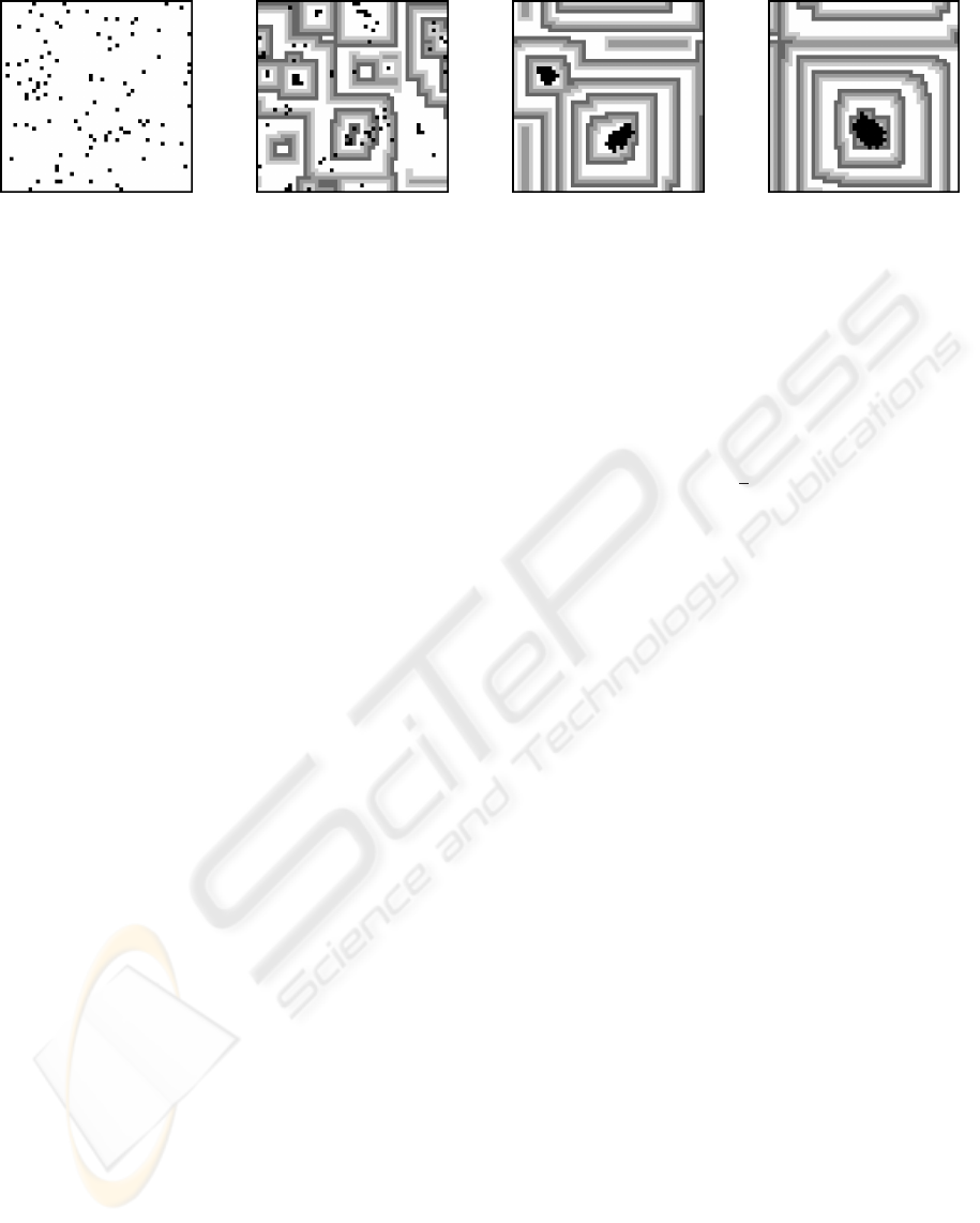
t = 0 t = 50 t = 500 t = 1500
Figure 3: Transactional CA simulation of a virtual amoebae gathering model. Under some environmental conditions, amoebae
(in black) release a morphogen (whose concentration is displayed as a gray scale). Then, they follow the gradient generated
by reaction-diffusion of that morphogen, until they all gather. Here, each environment patch contains up to two amoebae.
We have shown the interest of such an approach on a
diffusion-limited aggregation model allowing to find
the three steps required to synchronously run this
MAS in a CA framework. Then we proposed the
first step of a generalization and an automation of this
methodology. This work is based on the use of the
influence-reaction model that is naturally related to
the three-step approach of transactional CA.
Other solutions have already been proposed. For
example, specific kinds of CA have been designed
to model the movement of particles, like the dimer
cellular automata that develops an asynchronous
point of view of the dynamics, or the lattice gas
cellular automata initially developed for simulating
fluids (Deutsch and Dormann, 2005). The ques-
tion of coding moving objects in CA also led au-
thors to consider a two-step CA that prevents colli-
sions (Hochberger et al., 1999) or to extend the neigh-
borhood (Nishidate et al., 1996). This approach is
quite similar to a transactional CA. These solutions
focus on the displacement of objects and have not
been used yet in a more general context.
By contrast, transactional CA are developed in or-
der to consider any kind of action. For example, we
are currently applying the methodology presented in
section 4, to generate a CA corresponding to a model
of gathering virtual amoebae (Fat`es, 2008a), an illus-
trative MAS that involves an active environment to-
gether with a weak exclusion principle. As shown on
Figure 3, this result is promising and encourages us to
use our approach on a broader range of problems.
REFERENCES
Adamatzky, A. (2001). Computing in Nonlinear Media and
Automata Collectives. Institute of Physics Publishing.
Brooks, R. (1990). Elephants don’t play chess. Robotics
and Autonomous Systems, 6(1-2):3–15.
Chopard, B. and Droz, M. (2005). Cellular Automata
Modeling of Physical Systems. Collection Alea-
Saclay: Monographs and Texts in Statistical Physics.
Cambridge University Press.
Deutsch, A. and Dormann, S. (2005). Cellular Automa-
ton Modeling of Biological Pattern Formation Char-
acterization, Applications, and Analysis, volume 26
of Modeling and Simulation in Science, Engineering
and Technology. Birkh¨ı¿
1
2
user.
Fat`es, N. (2008a). Decentralised gathering on a discrete
field. Technical report, INRIA. http://hal.inria.fr/inria-
00132266/.
Fat`es, N. (2008b). Fiatlux CA simulator in Java.
http://webloria.loria.fr/ fates/fiatlux.html.
Ferber, J. (1999). Multi-Agent Systems, an Introduction to
Distributed Artificial Intelligence. Addison-Wesley.
Ferber, J. and Muller, J.-P. (1996). Influences and reaction:
a model of situated multiagent systems. In Proc. of
the 2nd Int. Conf. on MAS, pages 72–79.
Halbach, M. and Hoffmann, R. (2004). Implementing cel-
lular automata in FPGA logic. In Parallel and Dis-
tributed Processing Symposium, International.
Hochberger, C., Hoffman, R., and Waldschmidt, S. (1999).
CDL++ for the description of moving objects in cel-
lular automata. In Proc. of PaCT’99. Springer-Verlag.
Michel, F., Beurier, G., Gouaˆıch, A., and Ferber, J. (2003).
The turtlekit platform: Application to multi-level
emergence. In ABS 4 Agent-Based Simulation 4.
Nishidate, K., Baba, M., and Gaylord, R. J. (1996). Cellu-
lar automaton model for random walkers. Phys. Rev.
Lett., 77(9):1675–1678.
Regelous, S. (2004). MASSIVE: Multiple agent
simulation system in virtual environnement,
http://www.massivesoftware.com/.
Resnick, M. (1994). Turtles, termites, and traffic jams: ex-
plorations in massively parallel microworlds. MIT
Press, Cambridge, MA, USA.
Witten, T. and Sanders, L. (1981). Diffusion-limited aggre-
gation, a kinetic critical phenomena. Phys. Rev. Lett.,
47(19):1400–1403.
FROM REACTIVE MULTI-AGENTS MODELS TO CELLULAR AUTOMATA - Illustration on a Diffusion-Limited
Aggregation Model
429
