
RELAXATION OF SOCIAL COMMITMENTS IN MULTI-AGENT
DYNAMIC ENVIRONMENT
Ji
ˇ
r
´
ı Vok
ˇ
r
´
ınek, Anton
´
ın Komenda and Michal P
ˇ
echou
ˇ
cek
Gerstner Laboratory - Agent Technology Center
Department of Cybernetics
Faculty of Electrical Engineering
Czech Technical University
Technick
´
a 2, 16627 Praha 6, Czech Republic
Keywords:
Social Commitments, Multi-Agent Planning, Relaxation, Uncertainty.
Abstract:
The role of social commitments in distributed, multi-agent planning and plan execution will be discussed in
this article. We argue agents’ capability to reason about the actions in the form of social commitments directly
improving robustness of the plans in dynamic, multi-actor environment. We focused on relaxation decommit-
ment strategy, targeted specifically to the time interval in which the agent agrees to accomplish the commit-
ment. We will discuss how changes of this interval affect the plan execution and how the potential changes
of this interval can be represented in the commitment itself. The value of the use of social commitments in
planning in dynamic, multi-actor environment has been documented on a series of empirical experiments.
1 INTRODUCTION
Cooperation between intelligent agents is usually es-
tablished by means of negotiation resulting in a set of
obligations for the participating agents that lead on-
wards to achievement of a common goal agreed to
by the agents. Wooldridge and Jennings formalize
the obligations by describing the cooperative problem
solving by means of social commitments (Wooldridge
and Jennings, 1999) - the agents commit themselves
to carry out actions in the social plan leading onwards
to achievement of their joint persistent goal (Levesque
et al., 1990).
While classical planning algorithms produce a se-
ries of partially ordered actions to be performed by in-
dividual actors, we propose an extension of the prod-
uct (but also an object) of the planning process so that
it provides richer information about the context of ex-
ecution of the specific action. The context shall be
particularly targeted towards mutual relation between
the actions to be performed by individual actors and
shall be used mainly for replanning and plan repara-
tion purposes.
Each individual actor - when agreeing with task
implementation - adopts a commitment as a specific
mental state, which represents the actor’s proactive at-
titude towards goal implementation. The social com-
mitment contains the following pieces of information:
• commitment condition that may be (i) a specific
situation in the environment (such as completion
of some precondition) or (ii) a time interval in
which the action is to be implemented no mat-
ter what the status of the environment is or (iii)
a combination of both.
• decommitment conditions specifying under which
condition the actor is allowed to recommit from
the commitment once the task is finished (e.g. no-
tification) or once the task cannot be completed
(e.g. a failure)
Michael Wooldridge in (Wooldridge, 2000) de-
fines the commitments formally as follows:
(Commit A ψ ϕ λ),
λ = {(ρ
1
,γ
1
),(ρ
2
,γ
2
),...,(ρ
k
,γ
k
)},
(1)
where A denotes a committing actor, ψ is an ac-
tivation condition, ϕ is a commitment goal, and λ
is a convention. The convention is a set of tuples
(ρ,γ) where ρ is a decommitment condition and γ is
an inevitable outcome. The convention describes all
possible ways how the commitment can be dropped.
Generally speaking, the actor A has to transform the
world-state in such a way that the ϕ goal becomes true
if ψ holds and any γ has not been made true yet. The
520
Vok
ˇ
rínek J., Komenda A. and P
ˇ
echou
ˇ
cek M. (2009).
RELAXATION OF SOCIAL COMMITMENTS IN MULTI-AGENT DYNAMIC ENVIRONMENT.
In Proceedings of the International Conference on Agents and Artificial Intelligence, pages 520-525
DOI: 10.5220/0001662105200525
Copyright
c
SciTePress

actor is allowed to drop the commitment if and only
if ∃i : ρ
i
which is valid. A decommitment is allowed
provided that γ
i
is made true.
Decommitment strategies represent the main dis-
tinction between a commitment and an action as
a product of the multi-agent planning. The piv-
otal research problem when designing the multi-
agent commitments-based planning algorithm is in
designing agent’s capability to reason not only about
the actions, the conditions when the actions can
be implemented and the quality of service but also
about various decommitment rules and strategies to
be adopted by the agent who commits to imple-
mentation of the particular action. More informa-
tion about commitment-based planning in multi-agent
systems and decommitment strategies can be found
in (Komenda et al., 2008)
Another representation of commitments consider-
ing temporal account has been introduced in (Mallya
et al., 2003). CTL (Emerson and Srinivasan, 1988)
has been extended to capture features usually not con-
sidered in common approaches (but relevant for real-
istic environments), namely time intervals considered
in commitments satisfaction, “maintenance” manner
of commitments next to “achieve” manner of com-
mitments and vague specification of time. The un-
certainty in agent commitments has been studied in
(Xuan and Lesser, 1999). The authors have extend the
commitment by “... uncertainty by explicitly describ-
ing the possibility of future modification/revocation of
the commitment ...”. The focus has been put to the un-
certainty in the quality of the commitment fulfilment
(quality of service). Another aspects of commitments,
such as start time, finish time, or duration has not been
discussed.
In this article we will discuss the relaxation de-
commitment strategy based on Wooldridge’s commit-
ment representation, targeted specifically to the time
interval in which the agent agrees to accomplish the
commitment. We will discuss how these interval
changes affect plan execution and how the potential
changes of this interval can be represented in the com-
mitment itself. The value of the use of social commit-
ments in planning in dynamic, multi-actor environ-
ment has been documented on a series of empirical
experiments presented in Section 3.
2 RELAXATION IN
COMMITMENTS
The commitment time interval is usually captured by
the commitment subject ϕ and specifies the booked
time window for the commitment execution. The
temporal uncertainty can be a part of the commitment
subject definition (and thus the whole commitment
has to be renegotiated in case of any change) or, more
preferably, it can be included in the commitment as a
special instance of a decommitment rule.
Let the commitment time interval T
ϕ
= ht
s
,t
e
i,
where the t
s
is the starting time and the t
e
is the ending
time of the commitment time interval. The decommit-
ment rules can then be described as:
(Commit A ψ ϕ λ),
λ = {((t
est
s
6= t
s
) ∧ (t
est
s
∈ T
rlx
s
),t
s
= t
est
s
),
((t
est
e
6= t
e
) ∧ (t
est
e
∈ T
rlx
e
),t
e
= t
est
e
)},
(t
s
,t
e
) ⊂ ϕ,
(2)
where t
est
s
and t
est
e
are the estimations of the real start
and end of the activity and T
rlx
s
and T
rlx
e
are the agreed
relaxation intervals for the start and end time.
The t
s
, t
e
, T
rlx
s
and T
rlx
e
are the parameters of
the commitment negotiated and fixed in the planning
(contracting) time. The t
est
s
and t
est
e
are the agent’s es-
timates of the real start and end of the activity and can
vary in time.
The proposed representation of temporal uncer-
tainty in the commitment allows to allocate resources
(by the means of agent commitments - one agent re-
quests a resource that is provided by another agent)
accordingly in uncertain environment. In the mo-
ment of allocation (e.g. negotiation of the commit-
ment) the provider agent can make private estimation
of the possible future progress and setup the relax-
ation intervals without the need to reserve redundant
resources. The quality of estimation is the key issue
and affects the quality and robustness of the overall
plan. On the other hand, the requesting agent can se-
lect the provider according to the required flexibility
or stability of the commitment.
2.1 Impact on Planning and Negotiation
Planning using agent commitments is an optimiza-
tion method that takes into account individual goals
and constraints of the actors. The plan is constructed
by negotiation of agents, where the agents commit to
perform specific actions under the agreed conditions.
The key aspects of the negotiation are (i) establish-
ing commitments that are expected to be kept (mini-
mizing commitments violation) and (ii) minimize de-
commitment flexibility to avoid too much uncertainty.
Those two criteria are contradictory. In Section 2.2
we introduce a method that is focused on balancing
the flexibility and the stability of the commitments.
During the commitment execution, the agent is
able to update the estimations t
est
s
and t
est
e
for all future
commitments based on the current (and past) perfor-
mance and conditions. To enable propagation of this
RELAXATION OF SOCIAL COMMITMENTS IN MULTI-AGENT DYNAMIC ENVIRONMENT
521

information the decommitment rules (Equation 2) can
be extended with:
λ = {...,
((t
min
s
6= min(T
relax
s
)) ∧ (t
min
s
∈ T
rlx
s
),
T
rlx
s
= ht
min
s
,max(T
relax
s
)i)
((t
max
s
6= max(T
relax
s
)) ∧ (t
max
s
∈ T
rlx
s
),
T
rlx
s
= hmin(T
relax
s
),t
max
s
i)
((t
min
e
6= min(T
relax
e
)) ∧ (t
min
e
∈ T
rlx
e
),
T
rlx
e
= ht
min
e
,max(T
relax
e
)i)
((t
max
e
6= max(T
relax
e
)) ∧ (t
max
e
∈ T
rlx
e
),
T
rlx
e
= hmin(T
relax
e
),t
max
e
i)
}
(3)
In a complex interaction multi-agent scenario this in-
formation can help other agents to update their own
estimations and potentially improve their plans.
Equation 3 ensures that the commitment keeps
the previously agreed relaxation intervals but nar-
rows them down according to the updated informa-
tion. The relaxation intervals are updated to exclude
parts where the committed action is unlikely to be ex-
ecuted.
2.2 Relaxation Interval
This section describes the method for setting the com-
mitment relaxation interval inspired by the uncer-
tainty handling in the PERT
1
diagrams. The PERT
terminology operates with terms optimistic time, most
likely time and pessimistic time that incorporates the
uncertainty in the activity duration. Those terms are
used to compute the properties for each activity in the
project. In the network diagram representation, each
activity is described by its duration, early start, early
finish, late start, late finish and slack. Those param-
eters are very similar to the commitment representa-
tion of relaxation (the slack represents time reserve
and is not used in commitments). The original PERT
is usually used for a single project analysis, but set-
ting of the commitment relaxation in a multi-agent
system can be viewed from two points of view: (i)
the requestor agent (RA) that maintains the commit-
ments in the way similar to classical project manage-
ment and (ii) the provider agent (PA) that maintains
the commitments as independent entities agreed upon
with (potentially) various requestors.
The role of the requestor agent is to ensure con-
sistency between the dependent commitments consti-
tuted with particular provider agents. In this text we
are focusing on the provider agent, whose role is to
ensure commitments stability and flexibility with re-
spect to the environment uncertainty and resources
1
Program Evaluation and Review Technique
utilization. Those two points of view are very simi-
lar and the same strategies can be used for both.
The method of setting the relaxation interval pa-
rameters for i −th negotiated commitment is follows:
t
s
(i) = max(t
e
(i − 1),t
req
s
)
t
e
(i) = t
s
(i) +t
d
(i)
T
rlx
s
(i) = hmax(min(T
rlx
e
(i − 1)),t
req
s
),
max(max(T
rlx
e
(i − 1)),t
req
s
)i
T
rlx
e
(i) = hmin(T
rlx
s
(i)) +t
d
(i),
max(T
rlx
s
(i)) +t
d
(i) +t
r
∗ p
worst
b
(i)i,
(4)
where t
req
s
(i) and t
req
e
(i) are the start and end times re-
quired by the RA, t
d
(i) is the nominal duration of the
respective action, p
worst
b
(i) is the worst case estimate
of probability of breakdown during the task execution
and t
r
is the reparation time of the resource.
The relaxation intervals defined by Equation 4
correspond to the classical PERT representation. In
the case where the breakdown events happen more
than once per one activity, the p
worst
b
(i) doesn’t repre-
sent the probability value, but rather the relative num-
ber of breakdown events during the commitment exe-
cution.
3 EXPERIMENTS
The experiments evaluate three methods of handling
uncertainty. The first method is based on statistical er-
ror evaluation and uses a constant safety margin with-
out use of commitment relaxation rule. Other two are
based on relaxation with different relaxation intervals
estimation.
The experiments were performed on the scenario
with one requester agent (RA) and one provider agent
(PA). The PA maintains a single resource that is used
for tasks execution. The task execution is interrupt-
ible and only one task can be executed at any given
time. The RA requests a set of 1000 tasks from the
PA. The PA makes allocation for the tasks and pro-
poses a commitment for each individual task. The
commitment includes the start time, end time and re-
laxation intervals. The duration of the task is t
d
= 10
seconds.
Environment uncertainty is modeled as a resource
breakdown with a variable breakdown mean time t
b
and reparation time of t
r
= 5 seconds. An event sim-
ulation has been performed for 1000 randomly gen-
erated sets of breakdown events for each experiment
setting. The commitment parameters were computed
as follows:
ICAART 2009 - International Conference on Agents and Artificial Intelligence
522

(M
1
): Constant – this method extends the duration
of the task by the relative reparation time com-
puted by the probability of the breakdown for each
task. The start time of the commitment t
s
(i) =
t
e
(i − 1) and the t
e
(i) = t
s
(i) + t
d
(i) + t
r
∗ p
b
(i),
where p
b
(i) is the probability of the breakdown
during the commitment execution.
(M
2
): Linear – this method doesn’t change the dura-
tion of the activity, so the t
s
(i) = t
e
(i − 1) of the
previous commitment and the t
e
(i) = t
s
(i) +t
d
(i).
The relaxation interval for the decommitment rule
is computed as described in Section 2.2.
Commitment parameters computation are based on
the estimation of breakdown mean time ¯e
est
= 15 and
known reparation time t
r
= 5 seconds. The p
worst
b
esti-
mation is set to ¯e
est
. We measure the robustness of the
commitments and the resource utilization (total ex-
ecution time) under various conditions generated by
several environment uncertainty models.
The uncertainty models have been generated using
three methods. Each method produces an event sets
with various properties of mean value ¯e and standard
deviation σ. The environment uncertainty models are
the following:
(U
1
): Deterministic – breakdown events are gener-
ated evenly with t
b
period. This method produces
constant ¯e = t
b
and σ = 0.
(U
2
): Gauss – generates a set with normal distribu-
tion with ¯e = t
b
, σ = t
b
/10 with a delay between
two subsequent events restricted to h0,2 ∗ t
b
i.
(U
3
): Uniform – generates a set of uniformly dis-
tributed events with ¯e = t
b
with a delay between
two subsequent events restricted to h0,2 ∗ t
b
i.
The experiments were run with ¯e value varied accord-
ing to Table 1. The random sets were generated uni-
formly in this interval to evaluate the robustness of the
commitment relaxation setting methods. Because of
the relatively small event sets, the generated pseudo-
random values don’t fit exactly to the desired param-
eters (especially mean time value). The real ¯e of each
set has been computed within the simulation run and
corresponds to the x-axis in the provided evaluation
figures.
Table 1: Properties of the breakdown distributions.
distribution ¯e(s) σ (s)
U
1
10 ∼ 20 0
U
2
10 ∼ 20 1.5
U
3
10 ∼ 20 8.66
3.1 Observations
The figures below show the number of violated com-
mitments, tardiness of the commitments, and total ex-
ecution time for all methods under various uncertainty
settings. The total execution time of all commitments
is
∑
t
d
(i) = 1500 seconds and represents the ideal ex-
ecution duration in breakdown-free environment. The
length of the plan represents the end time of the last
commitment for the M
1
method and the latest time
of the relaxation intervals for the M
2
method. The
plan length is influenced by the experiment settings
and in our case it lengthens the plan for both methods
by 50% (caused by the parameters ¯e, t
d
and t
r
).
During the simulation, the agents kept all the com-
mitments as agreed at the beginning. The experiments
show the impact of non-accurate estimation on the er-
ror mean time. As expected, both methods provide
good results when ¯e > ¯e
est
. When the breakdown
mean time is shorter, both methods start to generate
commitment violations.
Figure 2 shows the mean time influence on the
number of violations. The commitment is violated
when it cannot be finished within the agreed limits
(t
e
for M
1
and relaxation interval T
rlx
e
for M
2
). The
robustness of the method M
1
is very limited. It pro-
vides good results only for deterministic uncertainty
U
1
with ¯e ≥ ¯e
est
. When ¯e < ¯e
est
, all the commit-
ments are violated (Figure 2–a). The M
2
method pro-
vides better results in the left-hand part of the graph
( ¯e < ¯e
est
) because of greater safety margin (caused by
p
worst
b
) but still converges quickly to the 100% vio-
lated commitments. For normal uncertainty U
2
the
situation changes. The M
1
method fails in the entire
range of ¯e and there is a low amount of non-violated
commitments even in the range ¯e > ¯e
est
(see Figure
2–b). The M
2
method provides a minimal amount
of violated commitments in the region ¯e > ¯e
est
and
¯e ∼ ¯e
est
and the number of violated commitments
slowly grows in the range ¯e < ¯e
est
. In the case of
uniform uncertainty U
3
both methods fail (Figure 2–
c). The lowest number of violated commitments is in
the right-hand region and it goes from approximately
50% to more than 80% for ¯e = ¯e
est
. The method M
2
provides good results for ¯e ≥ ¯e
est
. The number of vi-
olations grows with descending ¯e. For ¯e = ¯e
est
the av-
erage number of violated commitments is about 50%.
The total execution time is presented in Figure
1. Commitment execution is not started before the
agreed time (t
s
for M
1
and the relaxation interval T
rlx
s
for M
2
), so the execution time mainly corresponds to
the number of violated commitments. In case of the
M
1
method, the minimal execution time is equal to the
plan length (1500). The M
2
method execution time
RELAXATION OF SOCIAL COMMITMENTS IN MULTI-AGENT DYNAMIC ENVIRONMENT
523
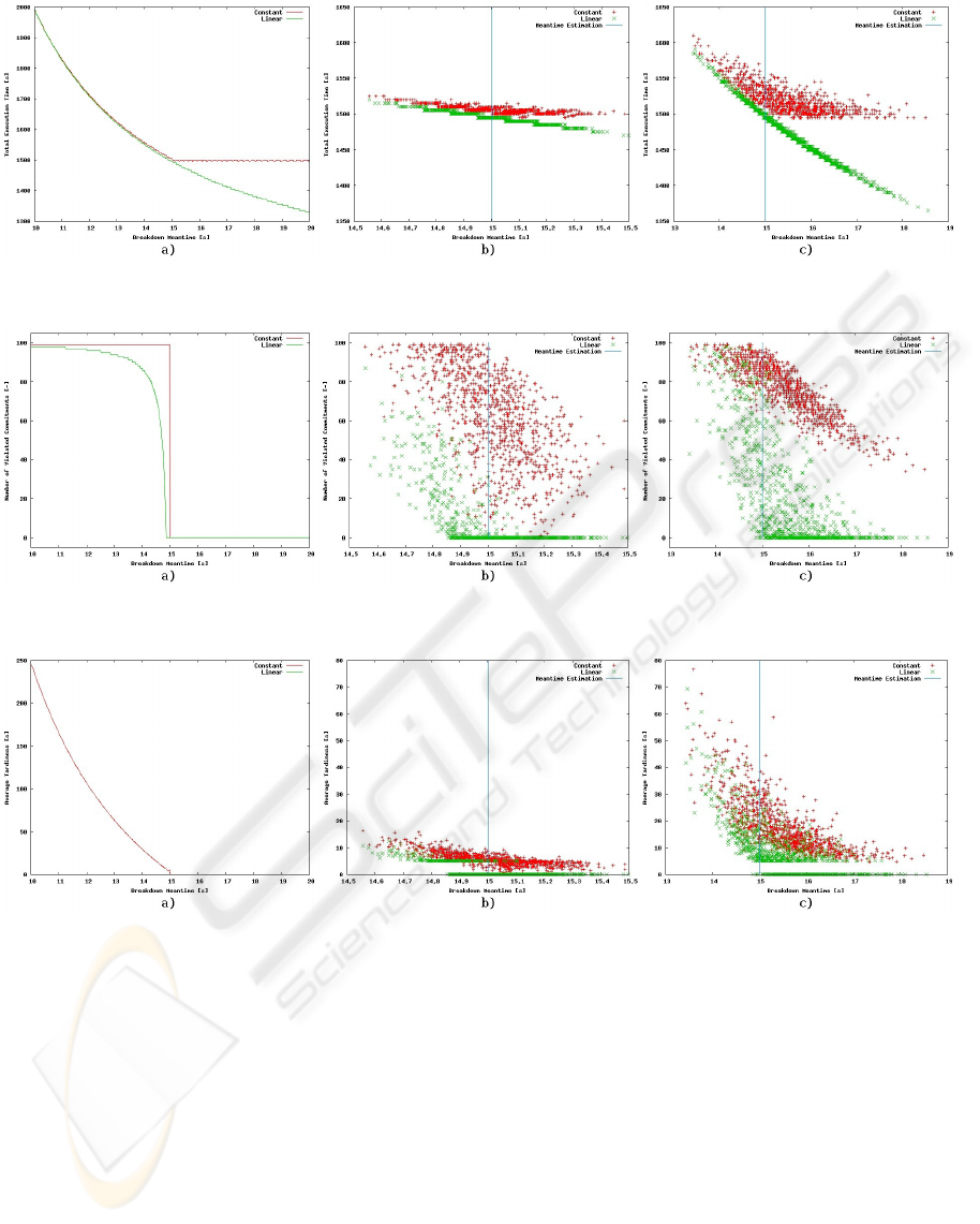
Figure 1: Total execution time with (a) deterministic mean time of breakdowns, (b) normally distributed mean time of break-
downs (¯e = t
b
, σ = t
b
/10), (c) uniformly distributed mean time of breakdowns.
Figure 2: Number of violations with (a) deterministic mean time of breakdowns, (b) normally distributed mean time of
breakdowns (¯e = t
b
, σ = t
b
/10), (c) uniformly distributed mean time of breakdowns.
Figure 3: Average tardiness with (a) deterministic mean time of breakdowns, (b) normally distributed mean time of break-
downs (¯e = t
b
, σ = t
b
/10), (c) uniformly distributed mean time of breakdowns.
converges to the
∑
t
d
(i) for the increasing ¯e.
For deterministic uncertainty U
1
both methods
provide hyperbolic growth of the total execution time
with decreasing ¯e (see Figure 1–a). The relatively
small difference between the methods is caused by the
fast growth of the violated commitments of method
M
2
and the low tardiness of the M
1
commitments
in the range where M
2
keeps the number of violated
commitments low. For normal uncertainty U
2
the total
execution time grows almost linearly with decreasing
¯e. The difference between the methods is given by the
difference in the number of violated commitments,
which is considerably higher for M
1
. For ¯e smaller
than the depicted value range, the execution time con-
verges to the execution time curve of the U
1
(as the
number of violations grows). The same situation oc-
curs for the case of uniform uncertainty U
3
. The dis-
ruption of the execution time curve of method M
1
is given by high variation of the number of violated
commitments. The total execution time of the M
2
is
similar to the total execution time for the other two
environment settings. The only difference is given by
small variation (±2% or less) of the execution time
for the particular ¯e. This variance depends on the vari-
ation of number of violated commitments for this ¯e
across the simulation runs.
The average tardiness of the commitment comple-
tion presented on Figure 3 is computed for all violated
ICAART 2009 - International Conference on Agents and Artificial Intelligence
524

commitments. The non-violated commitments are not
taken into account. If there is no violated commit-
ment, the average tardiness is set to zero. For deter-
ministic uncertainty U
1
the results of both methods
are very similar. The tardiness grows with decreas-
ing ¯e in a similar way as the total execution time. For
normal uncertainty U
2
both methods provide low tar-
diness that again converges to the curve for the U
1
environment setting for small values of ¯e (the conver-
gency is not captured by the Figure 3–b). Similarly to
the total execution length, the disruption of the curves
is given by the variation of the number of violated
commitments. For uniform uncertainty U
3
the aver-
age tardiness grows faster with the decreasing ¯e (see
Figure 3–c). The method M
1
provides relatively high
average tardiness of the commitments even in the re-
gion ¯e > ¯e
est
and ¯e ∼ ¯e
est
. The method M
2
provides
better results and the tardiness grows mainly in the
range ¯e < ¯e
est
.
4 CONCLUSIONS
We have presented the social commitment represen-
tation for multi-agent planning and plan execution
in the distributed domain with environment featuring
uncertainty. We have defined a relaxation decommit-
ment strategy targeted specifically to the time interval
in which the agent agrees to accomplish the commit-
ment. The relaxation strategy setting has been experi-
mentally evaluated and compared with a basic method
utilizing fixed commitments. The experiments have
proved that incorporating potential relaxation brings
certain benefits in comparison to the constantly eval-
uated safety margins.
The basic method M
1
is suitable mainly for de-
terministic environment U
1
where the relaxation de-
commitment strategy method M
2
brings no signifi-
cant improvement. Extending the safety margins in
both methods can scale the results towards lower ¯e but
lengthen the plans (and also the total execution time
for M
1
). For environments U
2
and U
3
, increasing the
safety margin brings no significant advantage because
of higher distortion of the breakdown distribution.
From the point of view of the number of violated
commitments, which is extremely important in the
multi-actors scenarios, the method M
1
fails for U
2
and
provides even worse results for U
3
. In this case, the
relaxation decommitment method M
2
is beneficial for
U
2
and keeps certain advantages even in U
3
, where
the average number of violated commitments is about
50%.
Another advantage of the M
2
method is its ro-
bustness. We have experimentally proved that the to-
tal execution duration and commitment tardiness does
not depend very much on the breakdown distribution
function (the results of experiments don’t differ by
more than 2%). With the increasing ¯e the total exe-
cution time converges to
∑
t
d
(i), which is the mini-
mal possible execution time. Due to the start time and
end time relaxation ability, the method enables both
optimistic and pessimistic execution without break-
ing the commitments. The relaxation decommitment
strategy greatly increases the flexibility, stability and
robustness of the agents’ social commitments in the
dynamic uncertain environment.
REFERENCES
Emerson, E. and Srinivasan, J. (1988). Branching time
temporal logic. In Linear Time, Branching Time and
Partial Order in Logics and Models for Concurrency,
School/Workshop, volume 354 of LNAI, pages 123–
172. Springer-Verlag.
Komenda, A., Pechoucek, M., Biba, J., and Vokrinek, J.
(2008). Planning and re-planning in multi-actors sce-
narios by means of social commitments. In Proceed-
ings of the International Multiconference on Com-
puter Science and Information Technology (IMC-
SIT/ABC 2008), volume 3, pages 39–45. IEEE.
Levesque, H., Cohen, P., and Nunes, J. (1990). On acting
together. In AAAI-90 Proceedings, Eighth National
Conference on Artificial Intelligence, volume 2, pages
94–99, Cambridge, MA, USA. MIT Press.
Mallya, A., Yolum, P., and Singh, M. (2003). Resolving
commitments among autonomous agents. In Dignum,
F., editor, Advances in Agent Communication. In-
ternational Workshop on Agent Communication Lan-
guages, ACL 2003, volume 2922 of LNCS, pages 166–
82. Springer-Verlag, Berlin, Germany.
Wooldridge, M. (2000). Reasoning about Rational Agents.
Intelligent robotics and autonomous agents. The MIT
Press.
Wooldridge, M. and Jennings, N. (1999). Cooperative prob-
lem solving. Journal of Logics and Computation,
9(4):563–594.
Xuan, P. and Lesser, V. R. (1999). Incorporating uncertainty
in agent commitments. In In: Proc. of ATAL-99, pages
221–234. Springer-Verlag.
RELAXATION OF SOCIAL COMMITMENTS IN MULTI-AGENT DYNAMIC ENVIRONMENT
525
