APPLYING Q-LEARNING TO NON-MARKOVIAN
ENVIRONMENTS
Jurij Chizhov and Arkady Borisov
Riga Technical University, 1 Kalku street, Riga, Latvia
Keywords: Reinforcement learning, Non-Markovian deterministic environments, Intelligent agents, Agent control.
Abstract: This paper considers the problem of intelligent agent functioning in non-Markovian environments. We
advice to divide the problem into two subproblems: just finding non-Markovian states in the environment
and building an internal representation of original environment by the agent. The internal representation is
free from non-Markovian states because insufficient number of additional dynamically created states and
transitions are provided. Then, the obtained environment might be used in classical reinforcement learning
algorithms (like SARSA(λ)) which guarantee the convergence by Bellman equation. A great difficulty is to
recognize different “copies” of the same states. The paper contains a theoretical introduction, ideas and
problem description, and, finally, an illustration of results and conclusions.
1 INTRODUCTION
One of the most topical tasks of artificial
intelligence is searching for optimal policy of
interaction with an environment by autonomous
intelligence software agent. Classical methods of
reinforcement learning are performing successfully
in the so-called Markovian environments. In this
work the idea and implementation approach are
stated for non-Markovian environments. The
approach offered represents a method of training
based on reinforcement learning. Thus it is
important to preserve the properties and advantages
of the classical algorithm of reinforcement learning
and its condition of convergence.
2 AGENT TASK AND
ENVIRONMENT
Reinforcement Learning (RL) is defined as the
problem of an agent that learns to perform a task
through trial and error interaction with an unknown
environment which provides feedback in terms of
numerical reward (Butz). The agent and the
environment interact continually (see Figure 1)
within discrete time. The experiments are carried out
in a well-known task - searching for a path in
labyrinth (kind of agent control), in other words,
building an optimal policy (strategy) of actions by
exploration of the environment. The reason for our
choice is obviousness and simple understanding of
the received results. SARSA(λ) learning algorithm
[Sutton] is preferred as a base learning algorithm,
which will be combined with the investigated
algorithms.
Figure 1: Agent-Environment interaction.
Let's consider the static cellular world - a
labyrinth. Each cell of the labyrinth is either free for
agent pacing, or occupied by some static obstacle.
One of the cells contains food (sometimes called
target cell or goal cell). In our case, the goal cell is
labelled by letter G. An example of simple grid
world is depicted in Figure 2.
To make the grid world usable like the
environment, we must define a set of data which
represent the state of the agent. Usually the state is
Agen
t
Environmen
t
action
t+1
s
t+1
next time-tick
reward state
a
t
r
t
s
t
306
Chizhov J. and Borisov A. (2009).
APPLYING Q-LEARNING TO NON-MARKOVIAN ENVIRONMENTS.
In Proceedings of the International Conference on Agents and Artificial Intelligence, pages 306-311
DOI: 10.5220/0001755603060311
Copyright
c
 SciTePress

all the information available to an agent that is
provided by its sensors. The set of agent sensors
(according to available information) depends on task
conditions. In our case the agent possesses only four
sensors: s
S
, s
E
, s
W
, and s
N
; each of them returns
value 1, if the obstacle is detected in a neighbor cell,
in the corresponding direction, otherwise value 0.
Thus, agent state might be expressed in binary form,
where each bit corresponds to each sensor. For
example, if the obstacle is North and East directions,
then state in binary form will be equal to S = 0101
2
.
For further calculation convenience, it is better to
convert the binary value to decimal form:
S = 0101
2
= 0·2
3
+ 1·2
2
+ 0·2
1
+ 1·2
0
= 5
10
Thus, on each step by getting values of sensors the
agent can compute the current state by formula 1:
S = 8·s
South
+ 4·s
E
as
t
+ 2·s
Wes
t
+ s
North
(1)
The value obtained is the state of the agent. Only
16 different states are available in our task
(including zero state interpreted as the absence of
obstacle around). Figure 2 depicts the grid world
with calculated values for each cell (state).
Figure 2: Grid world with evaluated states for each cell.
The agent can choose from four actions: to step
only one cell in each of four directions. It is
important to point out that each action of the agent is
surely executed. In other words, if in a previous state
s action a was applied, the probability of obtaining
next state s’ is equal to one: P(s, a, s’) = 1. If we
wish to use a probabilistic model for defining
probabilities of transitions, it requires including
additional 3-dimensional table.
Having a set of state, actions and probability of
transition, the grid-world-like environment now
might be represented in the transition graph form
which is often used for representing the Markovian
processes (Russell):
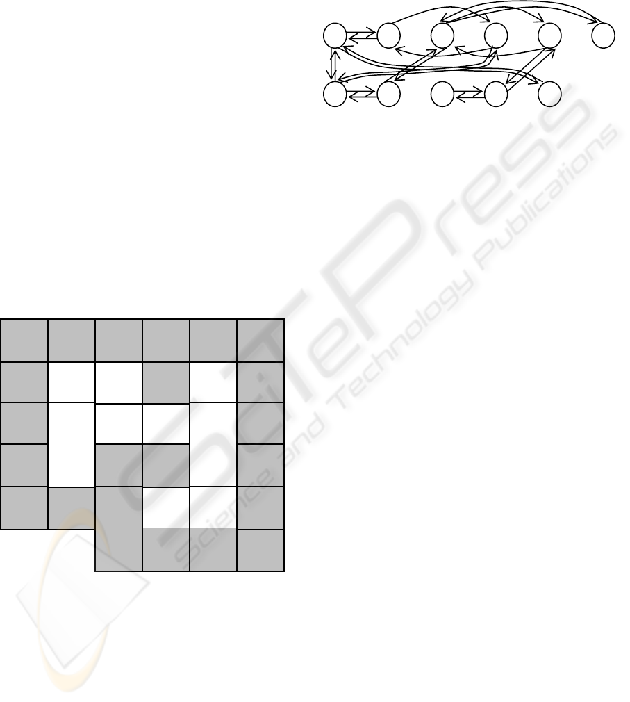
Figure 3: Agent environment in the graph form (states and
transitions form).
The arrows denote possible transitions through
implementing corresponding actions (moving north,
east, south and west). It is important to point out that
the grid world form is the form which is closer to the
real world form and keeps more properties than the
graph form. The graph form is a model which only
keeps information sufficient enough to the agent.
For example, looking at the grid world we can see
why a transition from one cell to another is
available. In graph mode we have only the fact of
available transitions. The reason might be
interpreted as additional information available for
operation. In our case the essential difference
between two forms is the properties that belong to
the nature of cell. Additional existence and the
number of non-Markovian states depend on the
precision of external world reproduction. Moreover,
the number of non-Markovian states might be
reduced by involving eight sensors instead of the
existing four. So, the graph representation is less
attractive than other forms; nevertheless it is worth
detailed consideration because of its representation
of state-action model, which is used in
reinforcement learning algorithms. In Table 1 the
main difference between grid-world form and graph
form is shown.
Two last distinctions cause the greatest interest.
These distinctions raise three fundamental problems
in the task of agent control in non-Markovian
environments:
1) detection of non-Markovian states;
2) detection of states with inconstant transition;
3) agent learning and its ability to distinct different
copies of the same states.
2 3 4 5
8 9
11
12
6
14
7
N
S
E
W
W
E
E
W
G
7
6
4
11
9 8
12
14
3
2
5
G
APPLYING Q-LEARNING TO NON-MARKOVIAN ENVIRONMENTS
307

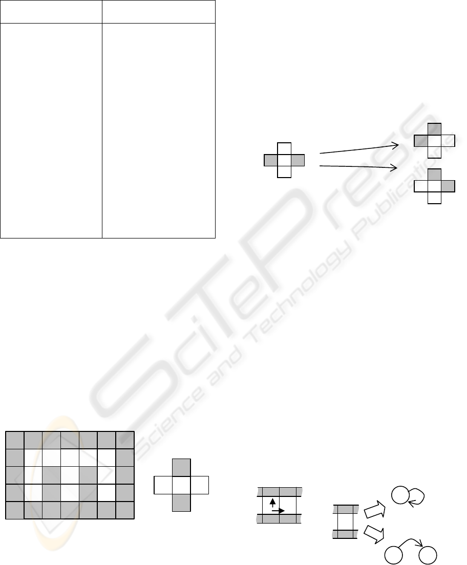
Table 1: Difference between two forms of environment
representation.
Grid world form Graph form
• The coordinate
system in the
labyrinth is caused by
the conception of cell
• Transitions move
the agent through
cells
• The obstacles and
cells arrangement
describes the actions
execution ability
• equally valued
state cells are
different copies of the
same state
•
there is no conception
of a cell, thus absence
coordinates
• transitions move the
agent from one state to
another
• there are no reasons
that could describe the
ability of executing
actions
• there is no conception
of the same state copies
,instead of that the
non-Markovian
conception or
inconstancy of transition
takes place.
3 THE SENSOR SIGNALS
INTERPRETING PROBLEM
As was mentioned above, in task of building optimal
policy through exploring non-Markovian
environment three problem cases might be revealed.
Case 1. The case supposes that from some state
at different moments of time it is necessary to
execute different actions. In other words, the current
state does not fully define the next action (Russell)
(Lin). This case is called non-Markovian state. The
Woods101 environment is a classical example of
such case (see Figure 4) (Kwee).
Figure 4: Left: Non-Markovian environment Woods101,
Right: an example of ambiguous state.
The cells denoted a and b, correspond to the
same state because of their equal values evaluated
upon agent sensors signals. Having appeared in that
state the agent sometimes is compelled to move east,
but sometimes west. Thus, having only current
state’s information, the agent is not capable of
making a decision and defining the optimal action.
Case 2 is the evolution of the previous and consists
of taking the same action from the same state at
different times, and the different reaction of
environment is observed. Let’s call this case the
transition inconstancy. Let’s see cells c and d, for
example. Again, each of them represents the same
state. An attempt to move north will lead to different
future states (see Figure 5).
Figure 5: Example of inconstant transition from state 6.
Case 3 relates to the problem of interpreting the
return of the same state (equal to source state). Let’s
consider state «9» depicted in Figure 6 (left). While
the agent is trying to move north, it meets the
obstacle, so, the environment returns agent to the
source (previous) state, which equals «9». Thus, two
ways of interpreting the situation are appropriate:
1) the agent was returned to the source state (see
Figure 6, right), or 2) the agent was moved to
another copy of the same state (like moving west or
east, see Figure 6, left). Different interpretations of
states are possible: either we do not take sensors
nature in account or instead of sensors methodology
the special channel for already evaluated state
transmitting is used. If the agent “understands” the
sensors meaning, it might be used as additional
signs. These signs might be sufficient to distinguish
different copies of the state. The model and agent-
environment conditions interaction are defined by
the task.
Figure 6: Left: fragment of an environment; Right: two
ways of interpretation.
c = d = 6 :
moving NORTH from state 6
like c leads to state 3:
moving NORTH from state 6
like d leads to state 5:
a = b = 9 :
d
G
b a
c
9 9
9
2
1
9
action
n
orth
9
actio
n
east
9’
ICAART 2009 - International Conference on Agents and Artificial Intelligence
308

The problem of distinguishing two equal states
is connected to that of representing same states in a
graph form or Markov chains. Should we duplicate
state «9» or leave it unique but having multiple
connections to neighbours? In its turn, there should
be «return links» which are responsible for agent
returning in source state in case of bumping to
obstacle.
4 SOLUTION
The idea of the solution in short is to build internal
Markovian representation of external non-
Markovian environment in parallel with learning
process. The solution includes the following tasks:
1) the problem of detecting non-Markovian states
and inconstant transitions;
2) the problem of conversion of ambiguous states
to Markovian states, more specifically:
a. problem of distinguishing exemplars of
same states;
b. problem of building internal representation
of the environment.
3) problem of agent learning and functioning in
external non-Markovian environment through
internal Markovian representation.
Hence, the implementation supposes the
following steps:
1) Develop an algorithm for detecting ambiguous
states.
2) Develop an algorithm for converting external
states to internal.
3) Slightly modify the existing Q-learning
algorithm for learning and controlling the agent
in internal environment.
4) Execute a number of experiments in most
famous non-Markovian environments, like
Woods101, Woods102, Maze5, Maze6, Maze7,
Maze10 etc.
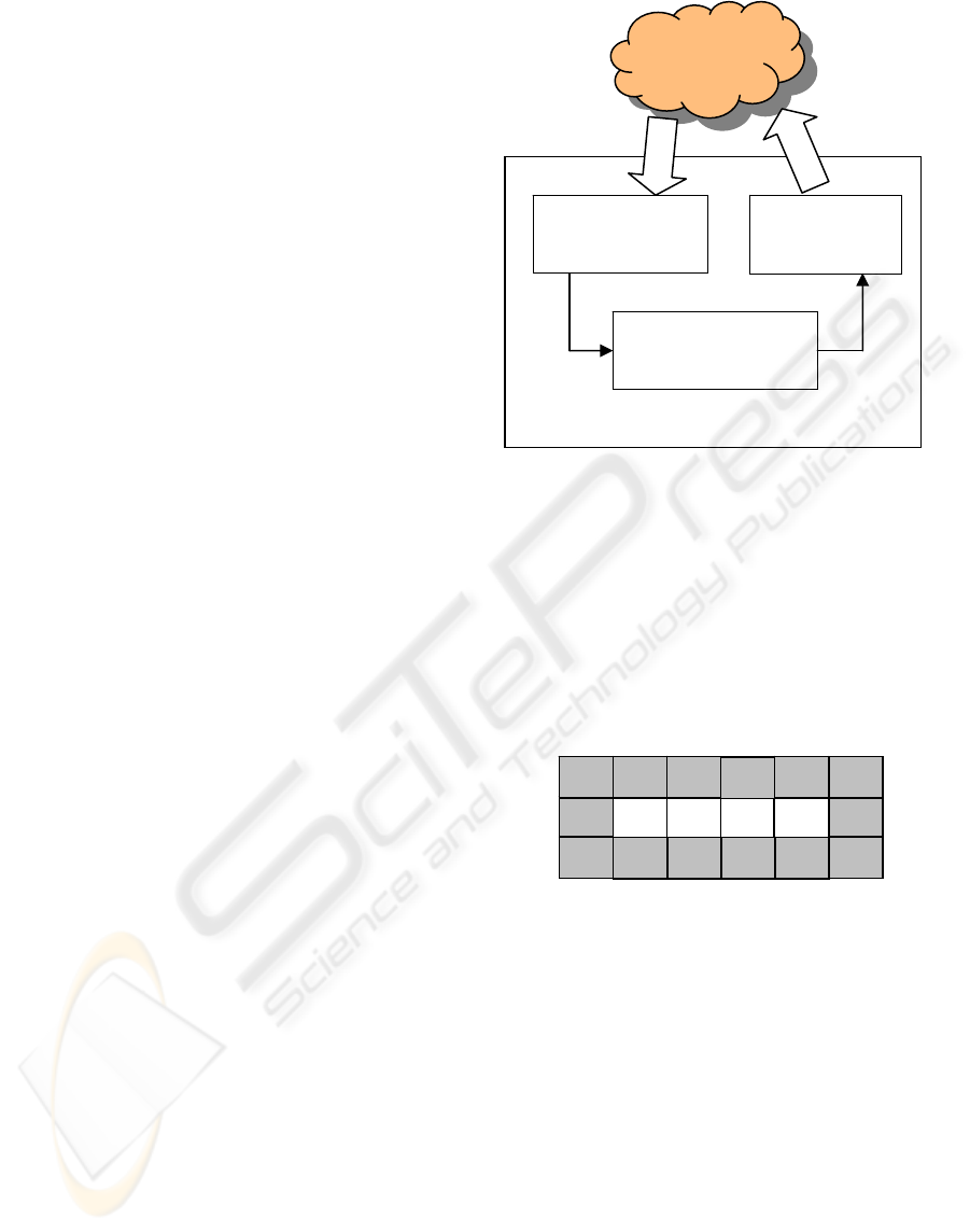
The general interaction architecture is depicted
in Figure 7. The architecture is based on the agent-
environment interaction model described in (Russel)
and (Padgham). It is important to point out that the
involved Sarsa(λ) algorithm (mentioned in (Sutton)
remains the same. It is necessary to guarantee the
convergence of algorithm. Only inessential
modifications are applied.
Figure 7: The general process.
4.1 The Indication of Ambiguous State
and Algorithm for its Detection
Non-Markovian states and states with inconstant
transition due to their common nature have common
simple indication: if transitions are observed when
the agent is moved from state s to different target
states by action a, then source state s is ambiguous.
A simple example is shown in Figure 8.
Figure 8: A simple example with ambiguous state «9».
During environment exploration, the agent finds
out that applying of action «step east» being in state
«11» always moves him to state «9». In its turn,
application of action «step east» being in state «9»
sometimes moves it to state «9» and sometimes to
state «13». Such an uncertainty makes the building
of the Q-table more difficult. The formal indication
of ambiguous state might be expressed as follows:
1''1
:),(:),(
++
≠
tt
ji
tt
ji
sassas
, (2)
where
t
ji
as ),(
and
'
),(
t
ji
as
are same corteges
observed at different moment of time,
1+t
S
and
1'+t
S
- states returned by the environment
(through sensors) at next time tick.
Converting to
internal state
S
i
REAL
ENVIRONMENT
state S
AGENT
Q-table possible
modification
Q-learning
execution
action a
9 13G 11 9
APPLYING Q-LEARNING TO NON-MARKOVIAN ENVIRONMENTS
309

Ambiguous state detection is executed within the
framework of Q-learning cycles and requires only
additional table size SxA for keeping observable
transitions. Each cell [s,a] keeps target state s’. As
soon next observation brings different target state,
the source state s is marked as ambiguous.
It is important to point out that the indication
does not require knowing of the goal state.
Ambiguous states detection occurs while Q-learning
builds its policy; it does not require special
exploration steps of the agent. For experiments the
algorithm was executed on a set of MacCallum’s
mazes and other environments. A short analyzing
log for each environment is presented in Table 2.
Table 2: Founded ambiguous states.
Maze
Founded ambiguous
states (state:action)
Woods101:
Maze5:
Maze7:
MazeT:
(6 :↑ )
(9: →)
(9: ←)
(1:→); (1:↓);
(1:←);
(2:→); (2:↓);
(2:↑);
(3:→); (3:↓);
(4:←); (4:↓); (4:
↑);
(5:←); (5:↓);
(6: ↑); (6:↓);
(8:→); (8:↑);
(8:←);
(9:→); (9:←);
(10:→); (10:↑);
(12:↑);
(6:↑);
(6:↓);
(9:→);
(9:←);
For the environment depicted in Figure 2 no
ambiguous states were detected. This result is true.
4.2 Making Internal Representation of
the Environment
Having a method for detecting ambiguous states, it
is time to build the internal representation. The L-
table (log) is used for storing the internal
representation of the environment. At the same time,
L-table is used for detecting ambiguous states. Each
row corresponds to a state. The columns represent
actions. For each action two columns are reserved.
The first column keeps the previous state. The
second one keeps next state. In the table below an
example of L-table is given.
Table 3: Example of L-table.
State
Departure state Arrival state
n e s w n e s w
1
9
11
13
14
9
11
16
1
16
1
9
16
1
9
14 9
11
16
16 |9 1 13 13 1
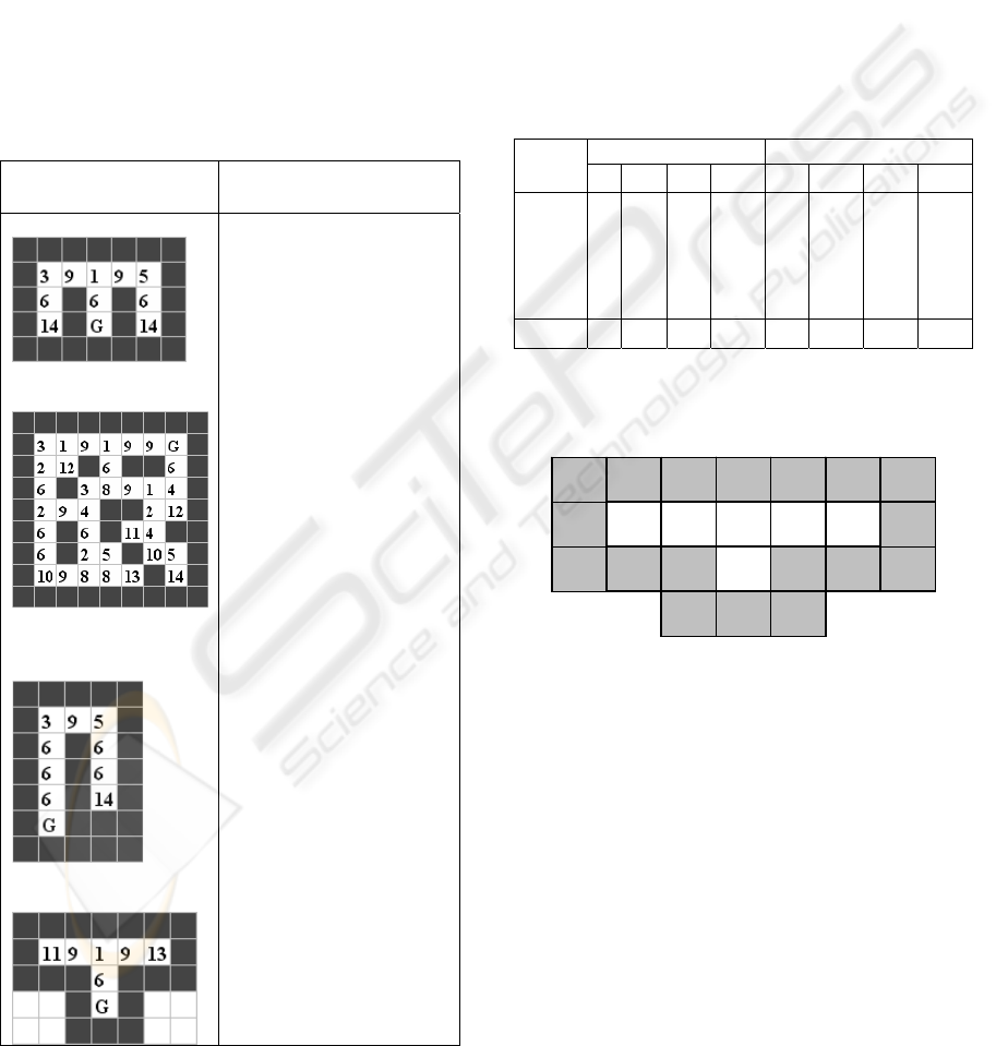
The L-table was built by the agent and contains
the internal representation of the environment
depicted in Figure 9.
Figure 9: Environmet with internal state «16».
The visible symmetry of L-table is only possible
in the task having contrary action like stepping left
and right or up and down, etc. To describe the
process of the table formation, let us consider state 1
in detail. Each “Departure state” means the state
where appropriate action was applied by the agent
with the following move to the current state 1 (row
1) Each “Arrival state” means the state, in which
agent will be moved after applying the appropriate
action from the current state 1. Actually, the L-table
is a form of memory (of depth one) storing the
applied action. The L table is filled by the agent
through the exploring of the environment. The
algorithm requires preliminary examination of the
problem of distinguishing exemplars of same states.
14
11 1 13 9 16|9
G
ICAART 2009 - International Conference on Agents and Artificial Intelligence
310

4.3 Distinguishing of Exemplars of
Same States
The main purpose of the internal representation is to
obtain dynamically created states. These states
represent each exemplar of the same original state as
a new state. In the L-table a new state is generated if
in filling the L-table a collision of states storing
occurs. For example, for the action east of state «9»
two destination states are possible: «1» and «13».
As soon as the collision appears, the new state will
be prepared and included in the table. In our case the
state «16» is descendant of state «9». Moreover, the
new state «16» inherits all appropriate transitions.
At the same time there arises a problem of
recognizing internal state having original external
state. The problem is solved by comparing the
transition history for one last step with the L-table. If
the L-table is not filled or filled partially, then
methods of random or directed selection are applied.
The algorithm under consideration is described
below. It is based on the original algorithm Sarsa(λ)
[Sutton]. The presentation is kept original. Only the
bold style is used to highlight the modifications
made and new elements introduced.
Initialize Q(s,a) arbitrarily and
e(s,a) = 0, for all s,a
Repeat (for each episode):
Initialize s, a, s
i
Repeat (for each step of episode):
Take action a, observe r, s΄
s΄
i
= GetInternal(s
i
, a, s΄)
IF isTransitionFickle then
Expand tables L, Q, e
s΄
i
is new one
Choose a΄ from s΄
i
using e-greedy
δ ← r + γQ(s΄
i
,a΄) – Q(s
i
,a)
e(s
i
,a) ← e(s
i
,a) + 1
for all s
i
,a :
Q(s
i
,a) ← Q(s
i
,a) + α δ e(s
i
,a)
e(s
i
,a) ← γ λ e(s
i
,a)
s
i
← s΄
i
; a ← a΄
Update table L
until s
i
is terminal
The denotation of variables is also kept original,
only s
i
and s’
i
are internal mappings of appropriate
states. As can be seen, the changes are related to
involving the mechanism of internal representation
and Q-table adaptation. The key procedure
GetInternal() returns internal state according to
table L:
Input parameters:
s
i
, a, s΄
Creating of list of descendant states
of s’
Searching of equal transition entries
Possible cases:
No entries: return external state
One entry: return it
Several entries:
applying methods of random or
directed search.
In case of several entries the incorrect internal
state might be returned. This situation is similar to
action testing in reinforcement learning: incorrect
returns will disappear. Application of an algorithm
like bucket brigade might be helpful in this case.
5 CONCLUSIONS
The proposed modified Sarsa(λ) algorithm
implements the idea of environment internal
representation. The modified algorithm is able to
recognize ambiguous states. Nevertheless, it suffers
from the lack of recurrent mechanisms to cope with
difficult mazes like Maze5 due to similar sequences
of transitions. The success of applying it on simple
mazes like Woods101, Maze7, MazeT demonstrates
the ability of the agent to build the internal
representation of the environment and use it in
reinforcement learning instead of original algorithm.
An interesting direction for further research is to
upgrade the algorithm to enable it to cope with
complicated environments. Future research will also
address the formalisation and generalisation of the
algorithm discussed
REFERENCES
Butz, M.V., Goldberg, D.E., Lanzi, P.L., 2005. Paper:
Gradient Descent Methods in Learning Classifier
Systems: Improving CXS Performance in Multistep
problems, IEEE Transactions, Vol. 9, Issue 5.
Sutton, R., Barto, R., 1998.
Reinforcement Learning. An
Introduction.
Cambridge, MA: MIT Press.
Russell, S., Norvig, R. 2003,
Artificial Intelligence: A
Modern Approach
, Prentice Hall. New Jersey, 2
nd
ed.
Padgham, L., Winikoff, M., 2004.
Developing Intelligent
Agent Systems. A Practical Guide.
John Wiley &
Sons.
Kwee, I., Hutter, M., Schmidhuber J., 2001. Paper:
Market-Based Reinforcement Learning in Partially
Observable Worlds.
Lin, L-J., 1993, PhD thesis
: Reinforcement Learning for
Robots Using Neural Networks,
Carnegie Mellon
University, Pittsburgh, CMU-CS-93-103.
APPLYING Q-LEARNING TO NON-MARKOVIAN ENVIRONMENTS
311