
A NOVEL APPROACH FOR NOISE REDUCTION IN THE GABOR
TIME-FREQUENCY DOMAIN
Behnaz Pourebrahimi and Jan C. A. van der Lubbe
ICT Group, EEMCS Faculty, Delft University of Technology, The Netherlands
Keywords:
Noise reduction, Time-frequency transform, Gabor transform, Low-pass filter, Image features.
Abstract:
In this paper, a noise reduction technique is introduced based on the Gabor time-frequency transform. In the
proposed approach, noise is removed using low pass filters locally in the transform domain. Finding the cut-off
frequency for the low pass filters in such a way that image does not loose its features, is an important issue.
The optimal cut-off frequency of the low pass filters are computed in an iterative method for each sub-block of
the image. The followed approach, besides showing a good performance in removing noise, it also performs
well in preserving image features.
1 INTRODUCTION
In the literature, there are several image denoising
methods which are applied in spatial, transform, or
time-frequency domains (Buades et al., 2004)(Barthel
et al., 2003),(Wang et al., 2006).(Cristobal et al.,
1996). In the spatial domain a small mask is con-
volved with the image. This mask can be an aver-
aging filter, a mean or Gaussian filter. In the trans-
form domain, first the image is translated to the trans-
form domain, then it is multiplied by a low pass filter
and at the end by the inverse transformation, the en-
hanced image is obtained. In the transform domain,
noise in the grey levels of an image contributes heav-
ily to the high frequency components and the most of
the image energy is concentrated in the low frequency
components. Although, applying a low pass filter to
a noisy image in the transform domain reduces the
noise, at the same time it could eliminate some high
frequency components that are not related to noise
and weaken sharp transitions like edges. Furthermore,
the transforms which perform on the whole image, do
not take into account any spatial information where
the frequency components come from. Therefore,
noise reduction by low pass filtering in such domains
does not preserve the local information of the image
very well. Time-frequency transforms combine time-
domain and frequency-domain analysis and allow ob-
taining a revealing picture of the temporal localization
of the signal’s spectral components.
In this paper, we consider the Gabor time-
frequency transform (Gabor, 1946) as a noise reduc-
tion technique. The Gabor transform is considered
as the optimum case of the short time Fourier trans-
form (STFT) in which the window function is chosen
to have a Gaussian shape. This choice of the win-
dow function in the 2-D Gabor elementary functions
guarantees the lower bound of the joint uncertainty
(i.e. the 2-D Heisenberg inequality) in the two con-
joint spatial-frequency domains. We propose an algo-
rithm in which noise is suppressed by applying low
pass filters to Gabor coefficients locally. The algo-
rithm by finding the optimal cut-off frequencies for
low pass filters attempts to preserve local information
of the image. We compare the performance of our ap-
proach with two Gaussian and Kuwahara filters given
their optimal performances. We also compare our al-
gorithm with a wavelet based denoising method. The
results show a good performance of our approach re-
garding the noise suppression and also preserving the
image features like edges.
The paper is structured as follows. Section 2
gives an overview of 2D Gabor transform. We dis-
cuss noise reduction in the Gabor domain and intro-
duce our method in Section 3. The results of applying
our method to noisy Lena image and comparison with
other methods are presented in Section 4. Finally, we
conclude in Section 5.
2 2D DISCRETE GABOR
TRANSFORM
The Gabor transform is first proposed by Gabor (Ga-
bor, 1946) for one-dimensional signals to analyze
22
Pourebrahimi B. and C. A. van der Lubbe J. (2009).
A NOVEL APPROACH FOR NOISE REDUCTION IN THE GABOR TIME-FREQUENCY DOMAIN.
In Proceedings of the Fourth International Conference on Computer Vision Theory and Applications, pages 22-27
DOI: 10.5220/0001768000220027
Copyright
c
SciTePress

speech and audio signals and later extended by Daug-
man (Daugman, 1985) to two-dimensions. The Gabor
analysis is based on projecting a given signal/image
onto a family of shifted and modulated Gaussian win-
dow functions, which are called the ”Gabor elemen-
tary functions” or the ”Gabor basis functions”. The
corresponding projection coefficients are called the
”Gabor transform coefficients”. The use of such a
transform is motivated by the fact that Gabor elemen-
tary functions have an optimal localization property,
in the joint time (or spatial) and frequency domains.
This leads to optimal extraction of the textural infor-
mation from the images, which is an important fea-
ture for pattern recognition, segmentation, and image
analysis applications. Beside the optimal localization
property other benefits of the Gabor transform include
compatibility with the human visual system and en-
ergy packing capability, which leads to lower entropy
in the transform domain.
As proposed by Daugman (Daugman, 1988) for
image compression and analysis, the elementary
functions are described in the following manner:
G(x,y) = exp(−π[(x − x
0
)
2
α
2
+ (y − y
0
)
2
β
2
])
×exp(−2π∗ i[u
0
(x − x
0
) + v
0
(y − y
0
)]). (1)
where (x
0
,y
0
) are the spatial coordinates of the cen-
ter and (u
0
,v
0
) are the spatial frequency parameters.
α and β are the standard deviations of the elliptical
Gaussian along x and y. The deficiency of the Ga-
bor transform, is that the elementary functions are
not orthogonal. Therefore, there is no straightforward
method available for extracting these transform co-
efficients. If they were orthogonal, the extraction of
these coefficients could have been done easily by tak-
ing the simple inner product. Many approaches have
been proposed to find a method for extracting the Ga-
bor transform coefficients. In this paper, we use the
algorithm introduced in (Teuner and Hosticka, 1993)
to compute the Gabor coefficients. This algorithm is
essentially an FFT-based gradient descent approach.
Consider a discrete two-dimensional signal I(x,y),
such as a digitized image of size P ∗ Q. The image
is divided into sub-images, each with M ∗ N pixels
and centers located at x
m
,y
n
= mM,nN for integers
(m,n). The elementary functions, whose widths are
determined by the Gaussian envelope parameters α
and β in equation (1), are defined over a 2M ∗ 2N
spatial lattice cell. A complete set of Gabor elemen-
tary functions is defined for each sub-image (m,n) by
varying the spatial frequencies
{
u
r
,v
s
}
=
r
2M
,
s
2N
corresponding to the 2M ∗ 2N spatial lattice cell. The
parameter r and s take on even integer values, r =
0,2,4,...,2M − 2 and s = 0, 2, 4, ...,2N − 2, because
the sub-image size is M*N. The center of each ele-
mentary function coincides with that of a sub-image
and (1) can now be rewritten as:
G
mnrs
[x,y] = exp(−π[(x − mM)
2
α
2
+ (y − nN)
2
β
2
])
×exp(−2πi[
r(x − mM)
2M
+
s(y − nN)
2N
]).
(2)
Each Gabor elementary function is now uniquely
determined by the integer pairs (m, n) and (r,s) rep-
resenting the spatial center and frequency parame-
ters, respectively (Srinivasan et al., 1993). The Gabor
transform of a 2-D image can now be written as:
I (x,y) =
∑
m
∑
n
∑
r
∑
s
C
mnrs
G
mnrs
(3)
where C
mnrs
are Gabor coefficients. If there would ex-
ist the functions W
mnrs
that were orthogonal to G
mnrs
,
then the Gabor coefficients would be computed as fol-
lows :
C
mnrs
=
P−1
∑
x=0
Q−1
∑
y=0
I (x,y)W
mnrs
(x,y). (4)
where
W
mnrs
= W (x − mM, y − nN)e
−2π j
(
rx
M
+
sy
N
)
. (5)
and below equation shows the orthogonality condi-
tion:
P−1
∑
x=0
Q−1
∑
y=0
W
mnrs
(x,y)G
mnrs
(x,y) = δ
m
δ
n
δ
r
δ
s
. (6)
Equation (4) can be presented as follows:
C
mnrs
=
P−1
∑
x=0
Q−1
∑
y=0
[I (x,y)W (x − mM,y − nN)]e
−2π j
(
rx
M
+
sy
N
)
=
P−1
∑
x=0
Q−1
∑
y=0
I
0
(x,y)e
−2π j
(
rx
M
+
sy
N
)
.
(7)
The signal I
0
(x,y) can be interpreted as an image
I(x,y) windowed by localized Gaussian, which is
centered at the location (m,n) on the Gabor lattice. If
M and N are powers of two, and the width P and the
height Q of the array (x, y) are multiple integers of M
and N, the computation of (7) requires a P ∗ Q 2-D
FFT. With substitution D
m
=
P
M
and D
n
=
Q
N
,equation
(7) can be modified as follows:
A NOVEL APPROACH FOR NOISE REDUCTION IN THE GABOR TIME-FREQUENCY DOMAIN
23
(a) (b)
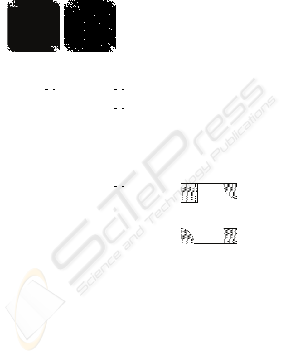
Figure 1: Power spectrum of an original image (a) and a
noisy image (b) in the Gabor domain.
P−1
∑
x=0
Q−1
∑
y=0
I
0
(x,y)e
−2π j(
rx
M
+
sy
N
)
=
M−1
∑
x=0
N−1
∑
y=0
I
0
(x,y)e
−2π j(
rx
M
+
sy
N
)
+
2M−1
∑
x=M
N−1
∑
y=0
I
0
(x,y)e
−2π j(
rx
M
+
sy
N
)
+
M−1
∑
x=0
2N−1
∑
y=N
I
0
(x,yt)e
−2π j(
rx
M
+
sy
N
)
+ ...
+
D
m
M−1
∑
x=M(D
m
−1)
D
n
N−1
∑
y=N(D
n
−1)
I
0
(x,y)e
−2π j(
rx
M
+
sy
N
)
=
M−1
∑
x=0
N−1
∑
y=0
I
0
(x,y)e
−2π j(
rx
M
+
sy
N
)
+
M−1
∑
x=0
N−1
∑
y=0
I
0
(x + M,y)e
−2π j(
rx
M
+
sy
N
)
+
M−1
∑
x=0
N−1
∑
y=0
I
0
(x,y + N)e
−2π j(
rx
M
+
sy
N
)
+ ...
+
M−1
∑
x=0
N−1
∑
y=0
I
0
(x + (D
m
− 1)M,y + (D
n
− 1)N)e
−2π j(
rx
M
+
sy
N
)
=
M−1
∑
x=0
N−1
∑
y=0
[
M−1
∑
D
m
=0
N−1
∑
D
n
=0
I
0
(x + D
m
M,y + D
n
N)]e
−2π j(
rx
M
+
sy
N
)
.
(8)
Hence FFT of an P ∗ Q image I
0
(x,y) followed by
decimation is substituted by M ∗ N point FFT, where
the FFT input signal I
0
(x,y) is calculated by summing
all points , equidistantly spaced about M and N. Re-
construction of the image can be done in the same
way by Gabor coefficients.
3 NOISE REDUCTION IN GABOR
TRANSFORM DOMAIN
In the Gabor domain, most energy of the image is
concentrated in a few coefficients. With computing
the Gabor transform of a N*N image using a N*N
Gaussian window, we observe that most of the im-
age energy has been concentrated in the low frequen-
cies. Figure 1 shows the image spectrum of an image
without noise and the corresponding noisy image in
the Gabor transform domain. From the figure 1(a),
we can see that the energy compaction of the image
spectrum is concentrated in the low frequency com-
ponents, while in a noisy image (figure 1(b)) energy
compaction is expanded in the whole image trans-
form domain. This energy packing property in Ga-
bor domain can be used for noise suppression. Such
as, eliminating high frequency components in trans-
form domain reduces the noise without loosing the
image information in low frequency components. A
low pass filter can eliminate the high frequency com-
ponents. Selecting the cut-off frequency of low pass
filter is important to make sure that no components
belonging to the image information is removed.
Figure 2 shows a N ∗ N low pass filter, chosen in
the Gabor domain. The low pass filter is selected ac-
cording to energy compaction of a N ∗ N image block
in the Gabor domain. The components in the dashed
area contain the most energy of the block. In this fig-
ure, x detects the harmonic border of the image spec-
trum. These regions have been chosen based on con-
jugated coefficients that have the same absolute val-
ues.
(
N
,x
-
1
)
(
N
,1
)
(
1
,
N
)
(1,x)
(1,
N
-
x
+
2
)
(x,1)
(
N
-
x
+
2
,1
)
(N
,
N
-
x
+
2
)
(N
,
N
)
(
N
-
x
+
2
,
N
)
(
x
-
1,
N
)
(1,1)
Figure 2: Low pass filter.
3.1 Proposed Noise Reduction
Algorithm
In this section, we introduce our noise reduction al-
gorithm. In the Gabor transform domain, the image is
analyzed through a Gaussian window whose dimen-
sions are smaller than the dimension of the image.
As already discussed, energy compaction of an image
in the Gabor domain is concentrated in the low fre-
quency components. So energy compaction in high
frequency components is related to noise. Using a
low-pass filter, we can save low frequency compo-
nents and eliminate the rest. Low pass filtering is per-
formed in the following manner: the Gaussian win-
dow is moved over the image and the Gabor transform
of the sub-image inside the window is calculated. Ga-
VISAPP 2009 - International Conference on Computer Vision Theory and Applications
24

bor components of the sub-image are filtered by a low
pass filter. Then by an inverse Gabor transform, the
enhanced sub-image is obtained. This procedure con-
tinues till the whole image is covered.
We assume that the dimension of the Gaussian
window is m ∗ m. c f is considered as the cut-off fre-
quency of the low-pass filter. The cut-off frequency
c f for each sub-image is calculated based on the max-
imum peak signal-to-noise ratios between different
versions of the enhanced sub-images with different
cut-off frequencies. We assume that the optimal cut-
off frequency is achieved when the peak signal-to-
noise ratio has its maximum value. Considering this
assumptions, the algorithm works as follows:
1. The Gaussian window is located at the coordi-
nates (1,1) of the image.
2. The block of the image inside the window is
named as x. Sub-image x is transformed to the
Gabor domain.
3. Cut-off frequency c f is initialized to c f = 1 and
variable psnr = 0 is set (psnr: peak signal-to-
noise ratio).
4. Gabor coefficients from step 2 are filtered by a
low-pass filter with the cut-off frequency c f .
5. Inverse Gabor transform is performed on the fil-
tered Gabor coefficients obtained from step 4 (the
new enhanced sub-image is named ex).
6. The peak signal-to-noise ratio (psnr) for two sub-
images x and ex are computed.
7. Cut-off frequency is increased (c f = c f +1). The
variable x is replaced with ex (x = ex). The steps
4-6 are repeated while c f < m/2 − 1.
8. The sub-image ex (from step 5) is selected as the
enhanced version of the original sub-image when
psnr has its maximum value (psnr(s) are com-
puted in step 6).
9. The Gaussian window is moved horizontally
along the image by f pixels (1 < f < m).
10. The values of the pixels in the overlapped areas of
the moving window are computed by averaging.
11. If end of the row is reached by the window, then
the window is moved vertically along the image
by f pixels (starting from left side of the image).
12. If the whole image is covered then the algorithm
stops, otherwise goes to step 2.
Table 1: Peak Signal to Noise Ratio (PSNR) in different
methods with two levels of Gaussian noise.
PSNR PSNR
σ
N
=25 σ
N
=50
Noisy Image 20.16 14.14
Enhanced Image (Gabor) 27.92 25.37
Enhanced Image (Kuwahara) 26.44 23.80
Enhanced Image (Gaussian) 28.91 26.41
4 PERFORMANCE EVALUATION
To evaluate the performance of our noise reduction al-
gorithm, we consider Lena image and apply the noise
reduction technique to its noisy version. The noisy
image shown in figure 3(a) has been corrupted by the
Gaussian noise with variance σ = 25. We compare
the performance of our approach with Gaussian and
Kuwahara filters. For each approach, we measure the
peak signal-to-noise ratio (PSNR) between the orig-
inal and enhanced image. The PSNR is calculated
based on the mean square error (MSE) between the
original and the enhanced image:
MSE =
1
M ∗ N
M
∑
i=1
N
∑
j=1
(I(i, j)− K(i, j))
2
(9)
PSNR = 10 log
10
(
p
2
MSE
) (10)
where I and K are the original and the noisy version
of an image with dimension M × N and p is the max-
imum possible pixel value of the image.
For our approach (in section 3.1), we applied the
algorithm with different sizes of the windows (m) and
different overlap values ( f ). We observed that the best
value for windows overlap is f = m/2. By applying
different sizes of windows, the best performance was
achieved for m = 16 and f = 8 in the most cases.
We considered a Kuwahara filter with the size
5×5. The Kuwahara filter is an edge-preserving filter
that smooths the noisy image but attempts to preserve
edges. With Gaussian filter, we tested with different
values for sigma. The results of applying the Gaus-
sian filter shown in this paper are the ones which have
given the highest peak signal-to-noise ratio (PSNR).
Table 2: Signal to Noise Ratio (SNR) in different methods
with three levels of Gaussian noise.
SNR SNR SNR
σ
N
=15 σ
N
=20 σ
N
=25
Noisy Image 18.75 16.25 14.29
Enhanced Image (Gabor) 24.02 22.92 22.06
Enhanced Image (WFW) 23.79 21.71 20.08
The enhanced images provided by applying the
three methods are shown in figure 3. The peak signal-
A NOVEL APPROACH FOR NOISE REDUCTION IN THE GABOR TIME-FREQUENCY DOMAIN
25
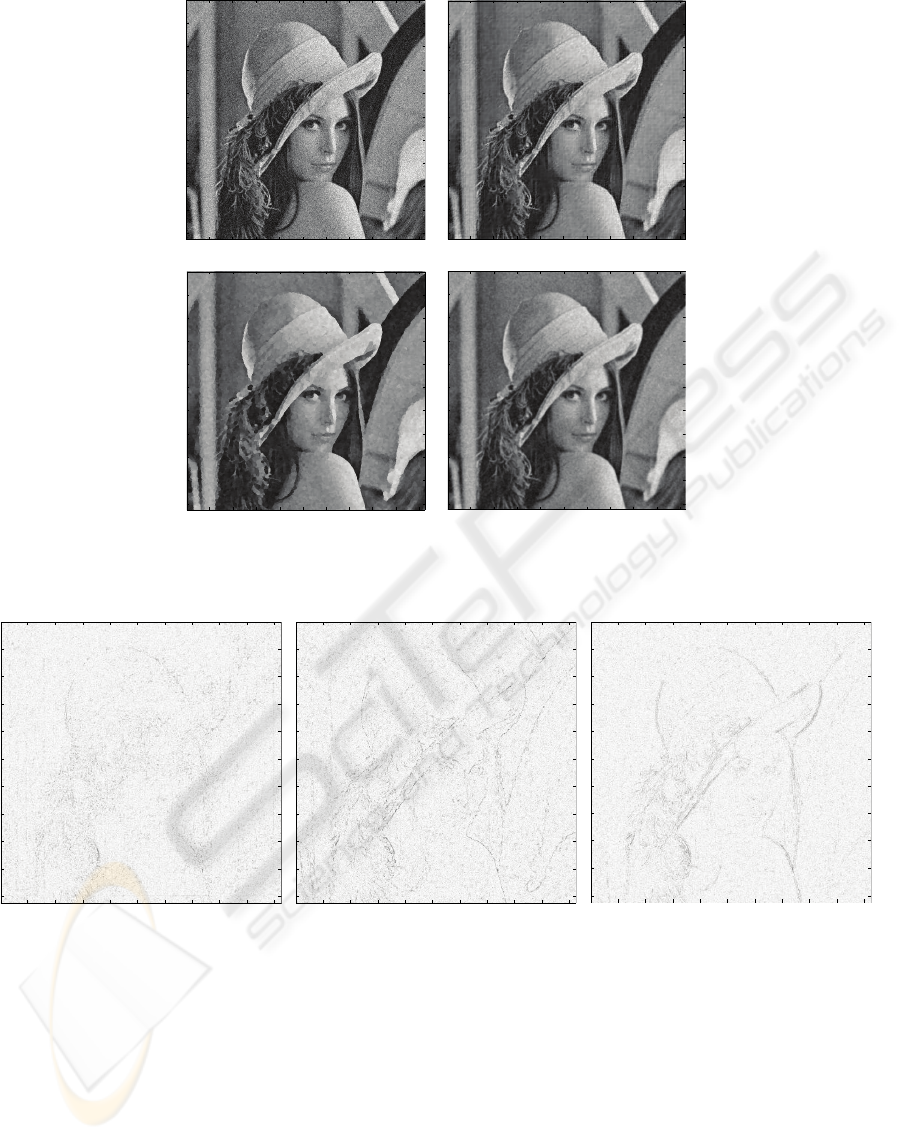
(a) (b)
(c) (d)
Figure 3: (a)Noisy image (Gaussian noise σ = 25), (b)Enhanced image using proposed algorithm (m=16, f=8), (c)Enhanced
image using Kuwahara filter (size=5 × 5), (d)Enhanced image using Gaussian filter.
(a) (b) (c)
Figure 4: Difference between noisy image and its enhanced version; (a)applying our method, (b)applying Kuwahara filter,
(c)applying Gaussian filter.
to-noise ratio (PSNR) is measured in each case and
is presented in table 1. Considering PSNR(s) in dif-
ferent approaches, the Gaussian filter shows the high-
est PSNR and Kuwahara filter the lowest. Let us re-
mark that the presented enhanced images with apply-
ing Gaussian and Kuwahara filters are selected given
the highest PSNR.
It should be taken into account that a higher PSNR
does not always guarantee a good visual quality of
the restored image. The PSNR by itself would not
be meaningful and the visual quality of the restored
image is also necessary to evaluate the performance
of denoising methods. To compare visual quality of
the enhanced images, we consider the subtraction of
enhanced image from its noisy version. The more
this difference looks like a real Gaussian noise, the
better the method is. In fact, this difference tells us
which geometrical features or details are preserved
VISAPP 2009 - International Conference on Computer Vision Theory and Applications
26

by the denoising process and which are eliminated.
Figures 4(a), 4(b) and 4(c) depict the difference be-
tween the noisy image and the denoised image using
our approach, Kuwahara and Gaussian approaches re-
spectively. The results show that our method preserve
more image features such as edges compared to other
two approaches. As, the difference of the noisy and
the enhanced image in our approach looks more like
Gaussian noise and contains less image features.
In the results shown above, we compared our algo-
rithm with two methods in spatial domain. In follow-
ing, we compare our method with a wavelet based de-
noising approach in time-frequency domain. We use
the results of the Wiener Filtering in the Wavelet do-
main (WFW) on noisy Lena image with different level
of Gaussian noise presented in (Wang et al., 2006).
As in this paper the results are shown based on mea-
suring signal-to-noise ratio (SNR), we also compute
the SNR when applying our method to the noisy im-
age with the same level of Gaussian noise. SNR is
computed as follows:
SNR = 10 log
10
(
∑
M
i=1
∑
N
j=1
S
0
(i, j)
2
∑
M
i=1
∑
N
j=1
(S
0
(i, j)− S(i, j))
2
) (11)
where S
0
is the noise free signal and S is the denoised
signal (Wang et al., 2006). Table 2 shows the results
for the two approaches. From the results, we can see
the our approach is also outperforming Wiener filter
in the wavelet domain. Our approach gives higher
signal-to-noise ratio for different level of noise.
5 CONCLUSIONS
In this paper, we have introduced a method for noise
suppressing in the Gabor time-frequency domain. In
the transform domain, high frequency components are
corresponding to the noise in the image. Consider-
ing this fact, the approach attempts to eliminate noise
with the low-pass filters which are located in the spa-
tial domain. In this way, the local information of the
image are preserved. The results of applying our ap-
proach to the noisy Lena image show good perfor-
mance compared with the spatial denoising methods
as well as a denoising method in the time-frequency
domain. The enhanced image provided by our ap-
proach, besides removing noise, shows a better qual-
ity in preserving image features compared to the ap-
proaches in the spatial domain.
REFERENCES
Barthel, K. U., Cycon, H. L., and Marpe, D. (2003). Image
denoising using fractal and wavelet-based methods. In
SPIE Proc, pages 10–18.
Buades, A., Coll, B., and Morel, J. M. (2004). On image
denoising methods. Technical report, Technical Note,
CMLA (Centre de Mathematiques et de Leurs Appli-
cations.
Cristobal, G., Chagoyen, M., Escalante-Ramirez, B., and
Lopez-Miranda, J. (1996). Wavelet-based denoising
methods. a comparative study with applications in mi-
croscopy. In SPIE Proc. Wavelet Applications in Sig-
nal and Image Processing IV, volume 2825, pages
660–671.
Daugman, J. G. (1985). Uncertainty relation for resolution
in space, spatial frequency, and orientation optimized
by two-dimensional visual cortical filters. J. Opt. Soc.
Am. A, 2(7):1160.
Daugman, J. G. (1988). Complete discrete 2-d gabor trans-
forms by nearal networks for image analysis and com-
pression. IEEE Trans. Acoustics, Speech and Signal
Proc., 36(7):1169–1179.
Gabor, D. (1946). Theory of communication. 93:429–457.
Srinivasan, V., Bhatia, P., and Ong, S. H. (1993). A fast
implementation of the discrete 2-d gabor transform.
Signal Process., 31(2):229–233.
Teuner, A. and Hosticka, B. J. (1993). Adaptive gabor trans-
formation for image processing. IEEE Transactions
on Image Processing, 2(1):112–117.
Wang, Z., Qu, C., and Cui, L. (2006). Denoising images
using wiener filter in directionalet domain. In CIMCA
’06: Proceedings of the International Conference on
Computational Inteligence for Modelling Control and
Automation and International Conference on Intelli-
gent Agents Web Technologies and International Com-
merce, page 228, Washington, DC, USA. IEEE Com-
puter Society.
A NOVEL APPROACH FOR NOISE REDUCTION IN THE GABOR TIME-FREQUENCY DOMAIN
27
