
OBJECT RECOGNITION USING MULTIPLE THRESHOLDING
AND LOCAL BINARY SHAPE FEATURES
Tom Warsop and Sameer Singh
Research School of Informatics, Holywell Park, Loughborough University, Leicestershire, LE11 3TU, U.K.
Keywords:
Object recognition, Multiple thresholding, Local shape features.
Abstract:
Traditionally, image thresholding is applied to segmentation - allowing foreground objects to be segemented.
However, selection of thresholds in such schemes can prove difficult. We propose a solution by applying
multiple thresholds. The task of object recognition then becomes that of matching binary objects, for which
we present a new method based on local shape features. We embed our recognition method in a system which
reduces the computational increase caused by using multiple thresholding. Experimental results show our
method and system work well despite only using a single example of each object class for matching.
1 INTRODUCTION
Object recognition methods have many applications
including; database image retrieval, landmark detec-
tion, manufactured part inspection, target identifica-
tion and scene analysis. In this paper, we are con-
cerned with providing a count and localization of dif-
ferent object types present in an image.
Objects extracted from an image can be classi-
fied, image thresholding can be used for such extrac-
tion. Typical use of image thresholding is that of im-
age segmentation, (Cao et al., 2002). For example,
(Chang and Wang, 1997) segment image grey values
into a desired number of classes by applying either
Guassian smoothing or high-pass filtering to the im-
age histogram, creating the desired number of valleys
in the histogram which are then used as thresholds.
(Cao et al., 2002) present a method for threshold se-
lection based on the maximum entropy theorem, uti-
lizing the probability of pixel value occurences in an
image. More recently, (Malisia and Tizhoosh, 2006)
apply Ant Colony Optimization, using ants to search
for low value grey regions. Image segmentation by
thresholding can be utilized for object extraction (Ri-
dler and Calvard, 1978). For example, (Kamgar-Parsi
and Kamgar-Parsi, 2001) present a method which ex-
tracts objects in infra-red images. Assuming objects
have a higher temperature than the background, local-
ising the area of greatest temperature provides the ob-
ject centroid area. Expanding this area and locating
the highest drops in heat provides the edge between
object and background. (Ridler and Calvard, 1978)
present an iterative method for the selection of sege-
mentation threshold. Whereby background samples
close to objects are used to determine the appropriate
threshold. The method presented by (Revankar and
Sher, 1992) uses a priori knowledge to determine if a
threshold should be used to segement thin lines from
an image or the entire object region. (Park, 2001)
present a method of selecting locally optimum thresh-
olds to segment vehicles from image backgrounds.
These locally optimum thresholds are selected by pre-
venting regions created merging and by preserving
the compactness of these regions. (S. Bhattacharyya
and Bandyopadhyay, 2002) describe a method of us-
ing thresholding to generate a region of interest in an
image which is, in turn passed to a Hopfield network
to extract the present object. More recently, (Yu Qiao,
2007) present a method to segment small objects from
a background, using the intensity contrast between
object and background.
Our method is different, producing multiple
thresholded versions and searching within these
thresholded versions. Figure 1 illustrates why this ap-
proach is adpoted. Figure 1(a) shows an image and
Figure 1(b) the corresponding histogram. This clearly
shows no single threshold can be computed for ob-
ject segmentation from the background. However, by
stepping through thresholds of the image, definite ar-
eas relating to the objects can be identified, Figure
1(c) - 1(d). This use of multiple thresholds is sim-
ilar to that presented by (Jiang and Mojon, 2003).
389
Singh S. and Warsop T.
OBJECT RECOGNITION USING MULTIPLE THRESHOLDING AND LOCAL BINARY SHAPE FEATURES.
DOI: 10.5220/0001770903890392
In Proceedings of the Fourth International Conference on Computer Vision Theory and Applications (VISIGRAPP 2009), page
ISBN: 978-989-8111-69-2
Copyright
c
2009 by SCITEPRESS – Science and Technology Publications, Lda. All rights reserved
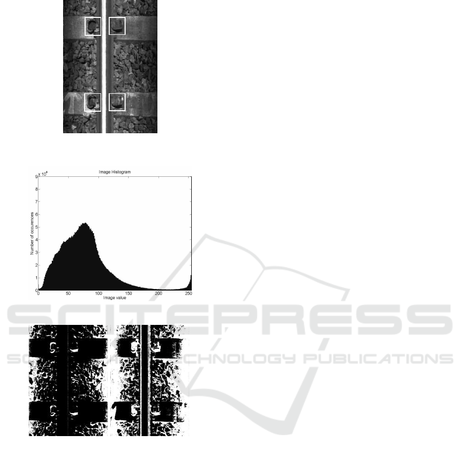
(a) Image with objects of
interest in white boxes
(b) Histogram of grey values in image (a)
(c) Threshold value
of 40
(d) Threshold value
of 70
Figure 1: Example image.
However, we counteract the computational increase
caused by processing multiple thresholded versions
of an image. First, image regions of interest are se-
lected, using an iterative area decomposition method.
Secondly, we embed the object recognition method in
a multi-resolution hierarchy, which have been shown
to be computationally efficient for image processing
problems, (Cantoni et al., 1991; Cantoni and Lom-
bardi, 1995). Finally, the system learns spatial re-
lationships between observed objects, allowing for
a more efficient search for objects in image space,
(Wixson, 1992).
Our method is presented in section 2. Experi-
mental setup and results are presented in section 3.
Finally, section 4 presents conclusions drawn from
these experiments.
2 METHOD
Our system is composed of three stages - training, im-
age pre-processing and object recognition.
2.1 Training
Ideal Template Creation. Templates are created by
a user, applying an arbitrary threshold to an ex-
ample of the object to be searched for.
Learning Spatial Relationships. The spatial rela-
tionships between objects are learnt from a set of
ground truthed images. We categorize these re-
lationships into one of four types - above, below,
left and right.
2.2 Image Pre-Processing
The image pre-processing phase creates multiple
thresholded versions of an input image and identifies
candidate areas. The following describes this process.
1. Initialise the list of areas (AreaList) with M
thresholded versions of the original image
(a) Read and store the area at the head of the
AreaList - area = Pop(AreaList)
(b) Calculate the horizontal (hp) and vertical (vp)
projections of area, dividing by the height
(height) and width (width) of area respectively.
(c) Replace all values in hp and vp which are either
above or below chosen upper or lower bounds,
respectively, with -1.
(d) If (Contains(hp, −1) or Contains(vp, −1))
i. Using the combination hp and vp, extract co-
ordinates representing bounding boxes seg-
mented by the elements set to -1 and Push
each bounding box onto AreaList.
ii. Goto step 2.
(e) Accept area as a candidate area.
(f) If AreaList is not empty, goto step 2.
2.3 Object Recognition
We compare two methods, a simple differencing
method which subtracts two binary images and our
new method which compares shapes created by white
pixels in a windowed neighbourhood.
VISAPP 2009 - International Conference on Computer Vision Theory and Applications
390
2.3.1 Simple Difference Method (SDM)
For each position in an area (A), a slice (I) the same
size as the template (T) used for comparison is ex-
tracted. The similarity between these is calculated as:
SD(I, T) = 1−
width
∑
i=0
height
∑
j= 0
ABS(I(i, j) − T(i, j))
width× height
(1)
where width and height are the width and height of I
and T. The highest value of SD(I, T) in A is taken as
the response.
2.3.2 Local Shape Matching Method (LSMM)
For each pixel in an area, a slice (I) of the
same size as a template (T) being matched is se-
lected. For every position of a white pixel in T,
(x
w
, y
w
), Neighbourhood
I
is the set of white pixels
in the region I(x
w
− K, y
w
− K) → I(x
w
+ K, y
w
+ K)
where K relates to the size of the window. Sim-
ilarly, Neighbourhood
T
is the set of white pix-
els in region T(x
w
− K, y
w
− K) → T(x
w
+ K, y
w
+
K). These neighbourhoods of pixels are compared
using the centroid and principal axis angle. If
(x
1
, y
1
), (x
2
, y
2
), ..., (x
N
, y
N
) are members of a neigh-
bourhood, the centroid ( ¯x, ¯y) is calculated as:
¯x =
1
N
N
∑
n=1
x
n
, ¯y =
1
N
N
∑
n=1
y
n
(2)
The principal axis angle through pixels in a neigh-
bourhood is calculated as (described in (Chaudhuri
and Samal, 2007)):
tan 2θ =
2
N
∑
n=1
(x
n
− ¯x)(y
n
− ¯y)
N
∑
n=1
[(x
n
− ¯x)
2
− (y
n
− ¯y)
2
]
(3)
The similarity between two neighbourhoods
(LSM(x
w
, y
w
, I, T)) is then calculated as:
1
2
(
| ¯x
I
− ¯x
T
| + | ¯y
I
− ¯y
T
|
V
+
Abs(θ
I
) − Abs(θ
T
)
2π
) (4)
where, V = 4K. Note, if Neighbourhood
I
is empty,
LSM(x
w
, y
w
, I, T) is set to 0. The similarity between
a template area and area slice is the average similar-
ity for every neighbourhood, centred around a white
pixel of T:
S(I, T) =
M
∑
m=1
LSM(x
m
, y
m
, I, T)
M
(5)
where (x
1
, y
1
), (x
2
, y
2
), ..., (x
M
, y
M
) are the white pix-
els in T. As with the simple difference method, the
highest value of S(I, T) in an area is taken as the re-
sponse for the corresponding area of the image.
2.3.3 Multi-Resolution Hierarchy
In the multi-resolution hierarchy, an object is
searched for at the lowest resolution. If the maximum
response achieved is greater than a predetermined ac-
ceptance threshold, the object is classified as found.
If the response is less than an acceptance threshold
but greater than a predetermined removal threshold,
the area is searched at the next highest resolution in
the hierarchy. If the response is less than a removal
threshold, search in the area stops.
2.3.4 Spatial Relationships
If an object is found, the spatial relationships are used
to generate image areas to search for more objects.
Since objects are expectedto appear in these areas, the
acceptance threshold is reduced. It should be noted
that results found in areas selected using spatial re-
lationships may themselves create more areas due to
different spatial relationships (the effects of reducing
the acceptance threshold are not cumulative).
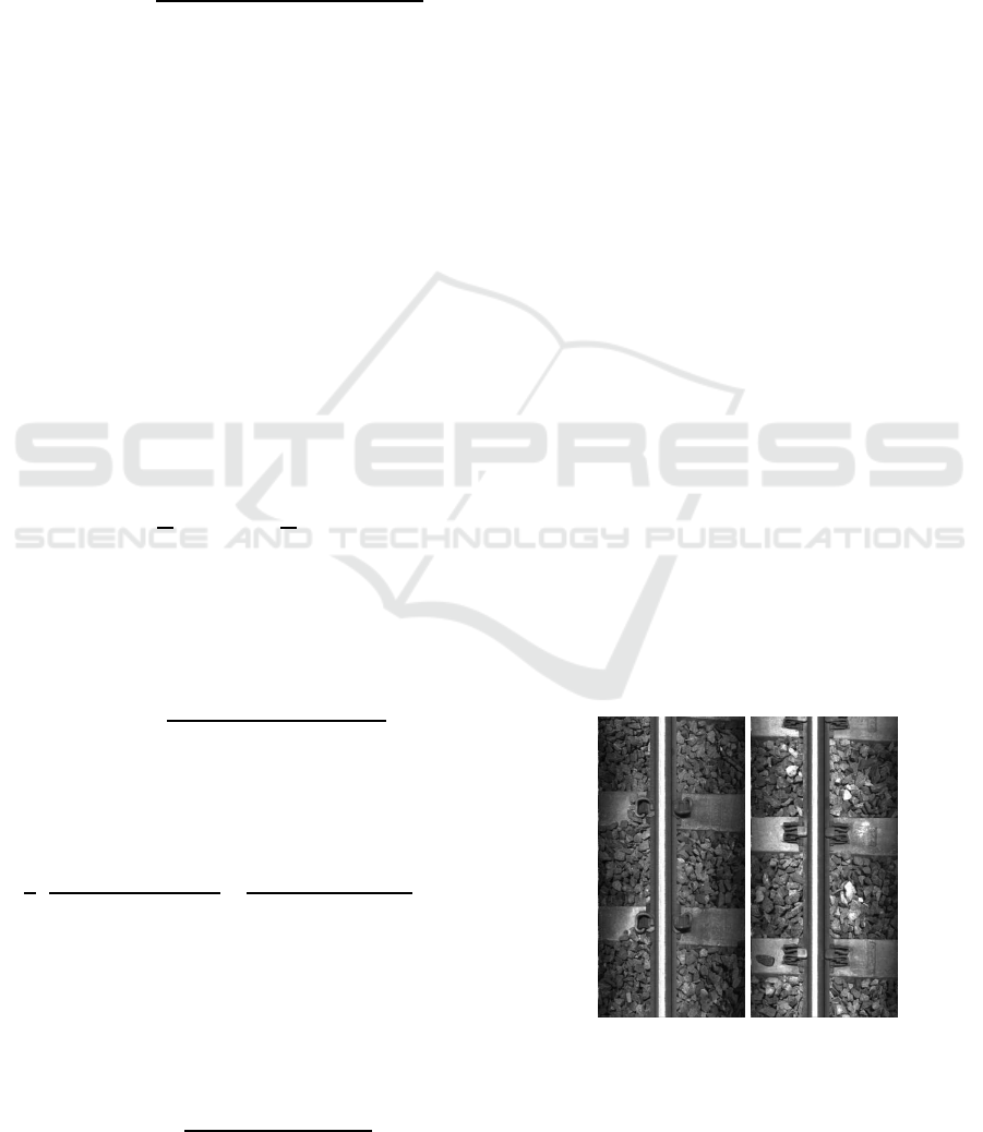
3 EXPERIMENTS
For experimentation, grey-scale input images were
taken from a camera looking down onto a rail track.
Examples of these images can be seen in Figure 2. A
total of 5000 images were used for testing. Within
these images, we search for instances of rail clips (ex-
amples shown in Figure 3).
(a) (b)
Figure 2: Example images.
OBJECT RECOGNITION USING MULTIPLE THRESHOLDING AND LOCAL BINARY SHAPE FEATURES
391
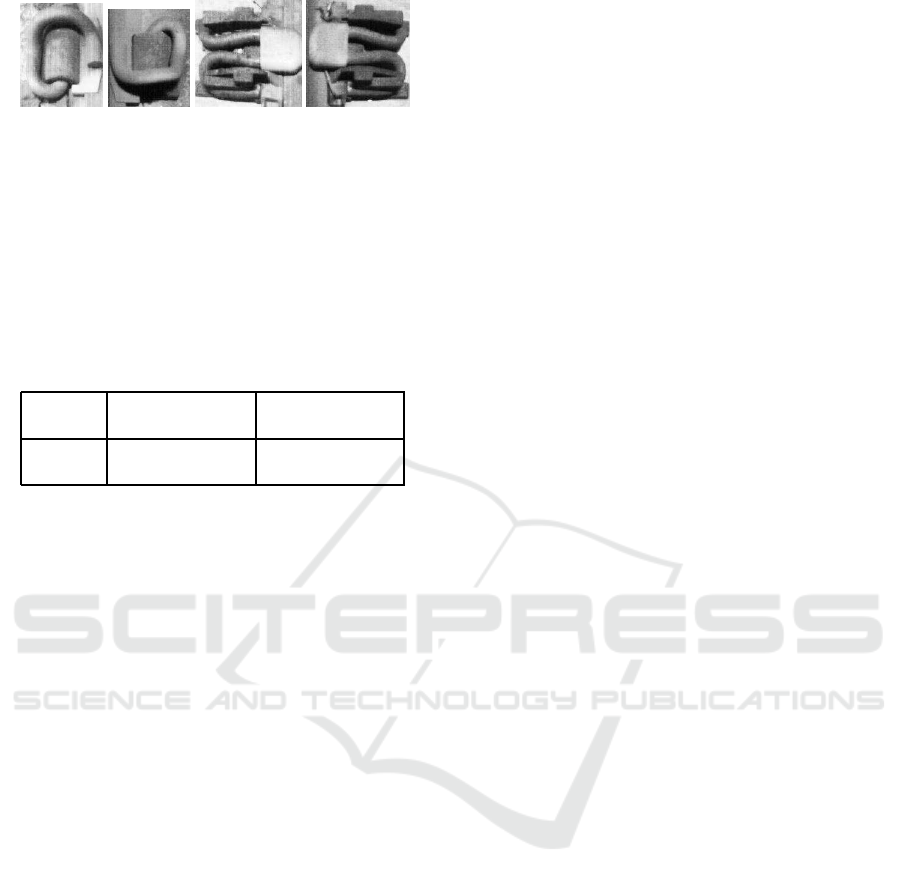
(a) (b) (c) (d)
Figure 3: Example objects.
The previously described object recognition sys-
tem was executed, using our data set, once using SDM
and once using LSMM. The results of which can be
found in Table 1. For each method, we show the cor-
rect percentage of objects found and the average num-
ber of false positives per image.
Table 1: SDM and LSMM results.
Method Percentage
Correct (%)
False Positives
per image
SDM 80.39 1.19
LSMM 91.6 0.16
Results show that LSMM outperforms SDM in
terms of average percentage of objects found and
number of false positives found. Note, without the
spatial relationship component in the system, LSMM
achieved an average recognition rate of 82.0% and a
similar number of false positives.
4 CONCLUSIONS
We have presented a method for object recognition
which achieves high recognition rates despite simi-
larities in grey-level values between objects and im-
age background. This was achieved by using a multi-
ple thresholding approach. For the object recognition
phase of our system, we presented a new local shape
matching method for binary objects, which performs
well despite using a single example of each object for
reference. We were also able to show that recogni-
tion performance can be enhanced through the use of
learnt spatial relationships between objects.
REFERENCES
Cantoni, V., Ferratti, M., and Lombardi, L. (1991). A com-
parison of homogeneous hierarchical interconnection
structures. In Proceedings of the IEEE, volume 79,
pages 416–428.
Cantoni, V. and Lombardi, L. (1995). Hierarchical architec-
tures for computer vision. In Euromicro Workshop on
Parallel and Distributed Processing, 1995. Proceed-
ings, pages 392–398.
Cao, L., Shi, Z. K., and Cheng, E. K. W. (2002). Fast auto-
matic multilevel thresholding method. In Electronics
Letters, volume 38, pages 868–870.
Chang, C.-C. and Wang, L.-L. (1997). A fast multilevel
thresholding method based on lowpass and highpass
filtering. In Pattern Recognition Letters, volume 18,
pages 1469–1478.
Chaudhuri, D. and Samal, A. (2007). A simple method for
fitting of boundary rectangle to closed regions. In Pat-
tern Recognition, volume 40, pages 1981–1989.
Jiang, X. and Mojon, D. (2003). Adaptive local threshold-
ing by verification-based multithreshold probing with
application to vessel detection in retinal images. In
IEEE Transactions on Pattern Analysis and Machine
Intelligence, volume 25, pages 131–137.
Kamgar-Parsi, B. and Kamgar-Parsi, B. (2001). Improved
image thresholding for object extraction in ir im-
ages. In International Conference on Image Process-
ing, volume 1, pages 758–761.
Malisia, A. R. and Tizhoosh, H.R. (2006). Image threshold-
ing using ant colony optimization. In Proceedings of
the 3rd Canadian Conference on Computer and Robot
Vision (CRV’06).
Park, Y. (2001). Shape-resolving local thresholding for ob-
ject detection. In Pattern Recognition Letters, vol-
ume 22, pages 883–890.
Revankar, S. and Sher, D. B. (1992). Pattern extraction by
adaptive propagation of a regional threshold. Techni-
cal report, University at Buffalo, State University of
New York, Dept. of Computer Science.
Ridler, T. W. and Calvard, S. (1978). Picture thresholding
using an iterative selection method. In IEEE Transac-
tions on Systems, Man and Cybernetics.
S. Bhattacharyya, U. M. and Bandyopadhyay, S. (2002). Ef-
ficient object extraction using fuzzy cardinality based
thresholding and hopfield network. In Indian Confer-
ence on Computer Vision, Graphics & Image Process-
ing.
Wixson, L. E. (1992). Exploiting world structure to effi-
ciently search for objects. Technical report, The Uni-
versity of Rochester.
Yu Qiao, Qingmao Hu, G. Q. S. L. W. L. N. (2007). Thresh-
olding based on variance and intensity contrast. In
Pattern Recognition, volume 40.
VISAPP 2009 - International Conference on Computer Vision Theory and Applications
392
