
A NOVEL APPROACH TO ORTHOGONAL DISTANCE
LEAST SQUARES FITTING OF GENERAL CONICS
Sudanthi Wijewickrema, Charles Esson
Colour Vision Systems, 11, Park Street, Bacchus Marsh 3340, Australia
Andrew Papli
´
nski
School of Information Technology, Monash University, Clayton 3800, Australia
Keywords:
Conic Fitting, Orthogonal Distance Least Squares Fitting.
Abstract:
Fitting of conics to a set of points is a well researched area and is used in many fields of science and engineer-
ing. Least squares methods are one of the most popular techniques available for conic fitting and among these,
orthogonal distance fitting has been acknowledged as the ’best’ least squares method. Although the accuracy
of orthogonal distance fitting is unarguably superior, the problem so far has been in finding the orthogonal
distance between a point and a general conic. This has lead to the development of conic specific algorithms
which take the characteristics of the type of conic as additional constraints, or in the case of a general conic,
the use of an unstable closed form solution or a non-linear iterative procedure. Using conic specific constraints
produce inaccurate fits if the data does not correspond to the type of conic being fitted and in iterative solutions
too, the accuracy is compromised.
The method discussed in this paper aims at overcoming all these problems, in introducing a direct calculation
of the orthogonal distance, thereby eliminating the need for conic specific information and iterative solutions.
We use the orthogonal distances in a fitting algorithm that identifies which type of conic best fits the data.
We then show that this algorithm requires less accurate initializations, uses simpler calculations and produces
more accurate results.
1 INTRODUCTION
Conic fitting is a well known problem and has ap-
plications in many fields. Among the methods avail-
able for this, the most common are: the Hough trans-
form (Hough, 1962), the moment method (Chaudhuri
and Samanta, 1991), and least squares fitting (Gauss,
1963). The two former methods become computa-
tionally inefficient when a higher number of param-
eters are involved, and hence, least squares methods
have received more attention in recent years. The ob-
jective of least squares fitting is to obtain the curve
that minimizes the squared sum of a defined error
measure.
min σ
2
=
n
∑
i=1
d
2
i
(1)
where, d
i
is the distance measure from of the i
th
point
and σ
2
is the squared sum of the errors over n points.
Depending on the distance measure that is
minimized, least squares fitting falls into two
main categories: algebraic and orthogonal (geomet-
ric/euclidian) distance fitting. The algebraic distance
from a point to a geometric feature (eg. curve or
conic) is defined by the following equation.
d
a
= f (p,x) (2)
where, p is the vector of parameters of the geometric
feature, x is the coordinate vector and f is the function
that defines the geometric feature or conic.
Although algebraic fitting is advantageous with
respect to computing cost and simplicity of imple-
mentation, it has many disadvantages, the most seri-
ous of which is the lack of accuracy and the bias of the
fitting parameters (Ahn, 2004; Fitzgibbon and Fisher,
1995). Changes have been suggested in an effort to
improve accuracy and one such error measure is the
first order approximation of the orthogonal distance
or the normalized algebraic distance (Taubin, 1991).
138
Wijewickrema S., Esson C. and PapliÅ
ˇ
Dski A.
A NOVEL APPROACH TO ORTHOGONAL DISTANCE LEAST SQUARES FITTING OF GENERAL CONICS.
DOI: 10.5220/0001771901370144
In Proceedings of the Fourth International Conference on Computer Vision Theory and Applications (VISIGRAPP 2009), page
ISBN: 978-989-8111-69-2
Copyright
c
2009 by SCITEPRESS – Science and Technology Publications, Lda. All rights reserved
d
n
=
d
a
k 5d
a
k
(3)
where, d
a
is the algebraic distance, d
n
is the normal-
ized algebraic distance and 5 =
∂
∂x
= [
∂
∂x
∂
∂y
]
T
Although using the normalized algebraic distance
gives better results than algebraic fitting, it also dis-
plays most of the drawbacks of the latter. In addition,
unlike algebraic fitting, it cannot be solved in closed
form, increasing the complexity of the calculations.
Orthogonal distance, which is agreed to be the
most natural and best error measure in least squares
techniques (Ahn, 2004), can be used to overcome
problems related to algebraic fitting. Although a
closed form solution exists for the calculation of the
orthogonal point for a general conic, numerical insta-
bility can result from the application of the analytic
formula (Fitzgibbon and Fisher, 1995; Press et al.,
1992). Therefore, either non-linear optimization tech-
niques for the general geometric feature (Ahn, 2004;
Boggs et al., 1987; Helfrich and Zwick, 1993) or
conic specific characteristics such as semi-axes, cen-
ter and rotation angle for ellipses (Ahn et al., 2001;
Gander et al., 1994; Spath, 1995) are used to calcu-
late the orthogonal distance.
In contrast, the algorithm discussed here employs
a novel and direct method of calculating the orthog-
onal distance, thereby overcoming the above men-
tioned problems. It also uses a simple procedure for
calculating the Jacobian matrix and determines the
best fit conic, irrespective of its type.
The rest of the paper is organized as follows: Sec-
tion 2 gives a brief review of conics and section 3 in-
troduces the proposed algorithm, while section 4 dis-
cusses experimental results.
2 REVIEW OF CONICS
A conic is expressed in the form of a 3 ×3 symmetric
matrix, C. If a point x = [x y 1]
T
, given in homoge-
neous coordinates is on the conic, it satisfies:
x
T
Cx = 0 (4)
where,
C =
˜
C c
c
T
c
=
c
11
c
12
c
13
c
12
c
22
c
23
c
13
c
23
c
33
, (5)
˜
C is a 2 × 2 symmetric matrix, c is a two element vec-
tor and c is a scalar.
We can extract the five independent parameters
of the conic from C by making c
33
equal to a con-
stant, assuming it’s not zero (for example, we use
c
33
= −1). Then, the parameter vector p is as follows:
270 272 274 276 278 280 282 284 286 288 290
166
168
170
172
174
176
178
180
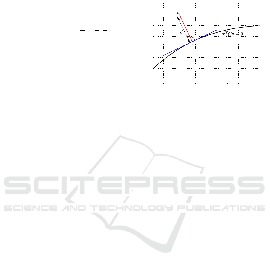
Figure 1: Orthogonal Distance between a Point and a Conic.
p = [c
11
c
12
c
13
c
22
c
23
] (6)
For any point x
p
not on the conic, there is a unique
line l
p
called the polar of the pole x
p
and is defined
as in equation (7) (Hartley and Zisserman, 2003). l
p
is the vector that satisfies the line equation l
p
T
x = 0
for any point x on it. If the pole x
p
is on the conic,
the polar l
p
becomes its tangent at x
p
(Semple and
Kneebone, 1956; Young, 1930).
l
p
= Cx
p
(7)
3 PROPOSED ALGORITHM
This section describes the orthogonal distance conic
fitting algorithm. First, in section 3.1, the orthogo-
nal distance is formulated, while its calculation is ex-
plained in section 3.2. Section 3.3 describes the com-
plete conic fitting algorithm.
3.1 Orthogonal Distance from a Conic
The orthogonal distance is the shortest distance from
a point to a conic, as shown in figure 1. The closest
point on the conic from the given point is called the
orthogonal point. Note that any point in space (on,
inside or outside the conic C) is represented by a, the
orthogonal distance by d, and the corresponding or-
thogonal point on C by x, and that the points are given
in homogeneous coordinates. For such a point a, the
orthogonal distance, is given by equation (8).
d =k
˜
x −
˜
a k (8)
where, a = [
˜
a 1]
T
,
˜
a = [a
1
a
2
]
T
, and
˜
x = [x y]
T
are
the non-homogeneous representations of the points a,
and x respectively.
Calculating the orthogonal distance involves the de-
termination of point x on the curve for a given point
A NOVEL APPROACH TO ORTHOGONAL DISTANCE LEAST SQUARES FITTING OF GENERAL CONICS
139
a. Since the orthogonal distance is the shortest dis-
tance from a point to a conic, the line connecting the
points x and a is normal to the conic at x. Therefore:
n
1
=
¯
Cx (9)
where, n
1
is the normal vector,
¯
C = [c
1
c
2
]
T
is the 2×
3 matrix formed by the first two rows of C, and c
1
and
c
2
are the first and second columns of C respectively.
The vector connecting the two points is given by n
2
=
˜
x −
˜
a = [x − a
1
y −a
2
]
T
. The same equation can be
written in the following form, to be consistent with
equation (9).
n
2
=
¯
Ax (10)
where,
¯
A = [a
1
a
2
]
T
, a
1
= [1 0 −a
1
]
T
, and a
2
=
[0 1 −a
2
]
T
.
Vectors n
1
and n
2
given in equations (9) and (10) are
in the same direction, and lead to equation (11).
¯
Cx = α
¯
Ax
=⇒
c
1
T
x
a
1
T
x
=
c
2
T
x
a
2
T
x
=⇒x
T
(c
1
a
2
T
− c
2
a
1
T
)x = 0
=⇒x
T
Bx = 0
(11)
where, B = c
1
a
T
2
− c
2
a
T
1
, and α is a scalar parameter.
The relationship obtained in equation (11) is that of a
conic, with one exception: the matrix representing the
conic B is not symmetric. Without loss of generality,
B can be manipulated to get the conventional form of
a conic matrix D, which is symmetric but also satisfies
the same relationship, as follows:
D =
B +B
T
2
(12)
Therefore, for the orthogonal point x of any point a,
the following equations are satisfied simultaneously.
x
T
Cx = 0
x
T
Dx = 0
(13)
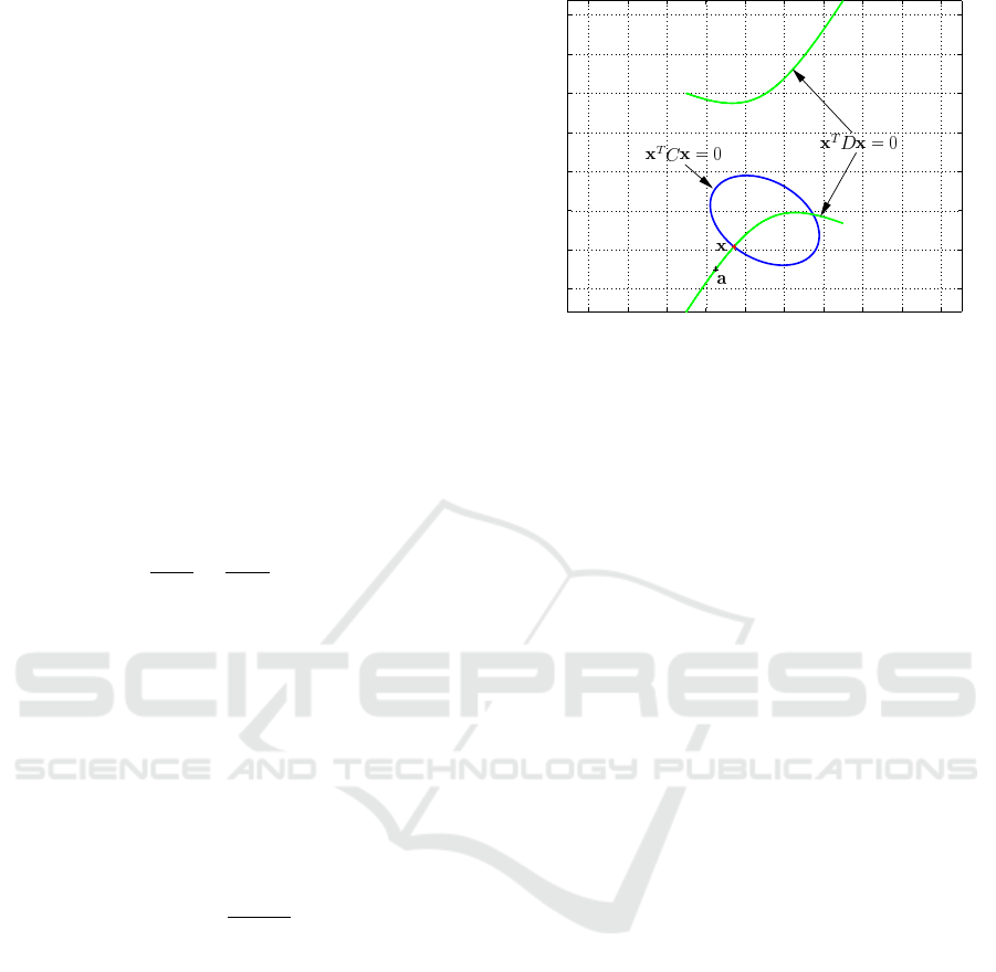
These two quadratic equations represent the intersec-
tion of two conics and is solved directly using the
method discussed in section 3.2. Out of the four pos-
sible solutions, the orthogonal point is the point clos-
est to a, a shown in figure 2.
3.2 Solving for the Orthogonal Point
To find the orthogonal point x, two quadratic equa-
tions with two parameters should be solved. This
results in the solution of a quartic equation whose
−60 −40 −20 0 20 40 60 80 100 120
−20
0
20
40
60
80
100
120
Figure 2: Orthogonal Point for a given Point on the Plane
with respect to a Conic.
closed-form solution is known to be numerically un-
stable (Fitzgibbon and Fisher, 1995; Press et al.,
1992). Therefore, iterative methods and/or the in-
troduction of conic specific information as additional
constraints are widely accepted as the norm in this
calculation (Ahn, 2004; Ahn et al., 2001; Faber and
Fisher, 2001). As explained above, this has undesir-
able properties such as complex calculations, and in-
accurate results when the fitted conic does not resem-
ble the distribution of the data points.
To overcome these problems, we use the method
used in (Miller, 1988) to solve for the intersection of
two conics, as discussed next. (Semple and Knee-
bone, 1956) and (Young, 1930) show that there exist
an infinite number of conics that go through the in-
tersection points of two conics, and that they can be
represented by a pencil of conics as follows:
C
f
= C + λD (14)
where, λ is a scalar parameter
(Semple and Kneebone, 1956) further explain that
there are three degenerate members (intersecting, par-
allel or coincident line pairs) in this pencil of conics,
and that they go through the common poles of C and
D. Like any member of the family, the degenerate
conics also share the common intersection points of C
and D. Equation (15) gives such a degenerate conic
and figure 3 illustrates the relationship between the
base conics and a degenerate member.
C
d
= C + λ
d
D (15)
where, λ
d
is the scalar that defines the degenerate
conic
To obtain the degenerate members, we need to cal-
culate the common poles of C and D. As shown by
(Semple and Kneebone, 1956), the three degenerate
members of a pencil go through one pole each, and
VISAPP 2009 - International Conference on Computer Vision Theory and Applications
140

−60 −40 −20 0 20 40 60 80
0
20
40
60
80
100
Degenerate
Conic
P
a
x
y
l
m
Figure 3: A Degenerate Member of the Conic Family.
therefore can be calculated by solving the general-
ized eigensystem (C − λD)x
p
= 0. This results in the
common poles (x
p
). We choose a finite, real common
pole out of these in our calculations. (Note that for
any point in space, an orthogonal point exists on the
conic C. Therefore, there exists at least one intersec-
tion point between C and D. This implies that we are
able to find at least one finite, real common pole to be
used in the calculation of the degenerate conic).
Since we know that C
d
goes through the chosen
common pole x
p
, it satisfies x
p
T
C
d
x
p
= 0. This gives
the value for λ
d
as shown in equation (16).
λ
d
= −
x
p
T
Cx
p
x
p
T
Dx
p
(16)
Now that C
d
is known, the next step is to extract
the line pair l and m that form it. The relationship be-
tween the lines and the conic matrix is given in equa-
tion (17). l and m can be extracted by using singular
value or eigen decomposition.
C
d
= lm
T
+ ml
T
(17)
Once the lines are obtained, the calculation of in-
tersection points is done by solving one of the conic
equations (x
T
Cx = 0 or x
T
Dx = 0) and the line equa-
tions (l
T
x = 0 and m
T
x = 0). This gives four solutions
(two each for the two lines), and we select the (real)
point closest to a as the orthogonal point. In figure 3,
x
p
is the common pole, x and y are the common inter-
section points of the pencil of conics and l and m are
the extracted lines.
3.3 Conic Fitting Algorithm
From the method discussed above, the orthogonal dis-
tance from the i
th
point (say a
i
) of a set of n points,
can be determined directly for a general conic. The
next step is to minimize the squared sum of all such
distances as shown in equation (1), to find the best fit
conic to the given set of points. Note that this is the
same quantity that is minimized in the distance based
algorithm of (Ahn, 2004) but assumes that the weight-
ing matrix or the error covariance matrix is identity
(Ahn et al., 2001). This results in an unconstrained
non-linear optimization procedure.
Out of the algorithms available for solving
this non-linear optimization problem, we select the
Levenberg-Marquardt method (Ma et al., 2004) due
to its robustness over other methods such as Gauss-
Newton. For each step of the iteration for the
Levenberg-Marquardt method, the update is done as
shown in equation (18).
p
k+1
= p
k
+ δ
δ
δ
k
(18)
where,
δ
δ
δ
k
= −(H
k
+ α
k
I)
−1
J
T
k
d
k
, (19)
J
k
is the Jacobian matrix for the k
th
step, H
k
= J
T
k
J
k
is an approximation to the Hessian matrix, I is the
5 × 5 identity matrix, δ
k
is the update vector, d
k
is the
orthogonal distance vector for all points at step k, and
α
k
is a scalar.
An initial guess for the parameter vector p
0
has to be
given, to start the iterative procedure. The selection
of this initial guess is done as discussed at the end
of this section. The values for the constant α
k
is ini-
tially set to a small constant (eg. α
0
= 0.01). For the
consequent steps, if the error increases or if the cal-
culated step yields an imaginary conic, the step is re-
peated with α
k
= n
const
×α
k
. If the error is decreased,
the next step is calculated with α
k
= α
k
/n
const
, where,
n
const
is a scalar constant (eg. n
const
= 10).
To calculate the Jacobian matrix for each step, in
the conventional way, it is required that the orthogo-
nal distance be expressed as a function of the conic
parameters. The method explained in section (3.1),
although very convenient for conics with known pa-
rameters, makes it difficult, if not impossible for those
with unknown parameters. Therefore, an alternative
method is used to find the Jacobian matrix, or the
matrix of first derivatives of the orthogonal distances
with respect to the conic parameters.
First, equation (8) is expressed in the form of
equation (20), the derivative of which, with respect to
the conic parameter vector p, leads to equation (21).
d
2
=k
˜
x −
˜
a k
2
= (
˜
x −
˜
a)
T
(
˜
x −a)
(20)
d
∂d
∂p
= (
˜
x −
˜
a)
T
∂
˜
x
∂p
(21)
Note that for each step, the orthogonal distance and
orthogonal point is known. Therefore, the only un-
knowns in equation (21) are
∂d
∂p
and
∂
˜
x
∂p
. To find values
A NOVEL APPROACH TO ORTHOGONAL DISTANCE LEAST SQUARES FITTING OF GENERAL CONICS
141

for the latter in terms of known quantities, the equa-
tions in (13) are differentiated with respect to the pa-
rameter vector p, resulting in:
2
x
T
C
x
T
D
∂x
∂p
= −
"
x
T
∂C
∂p
x
x
T
∂D
∂p
x
#
(22)
Since x = [
˜
x 1]
T
, equation (22) can be rewritten to get
equation (23).
2
x
T
¯
C
T
x
T
¯
D
T
∂
˜
x
∂p
= −
"
x
T
∂C
∂p
x
x
T
∂D
∂p
x
#
(23)
where,
¯
C and
¯
D are the 2 × 3 matrices consisting of
the first two rows of C and D respectively.
The solution of equations (21) and (23) gives an ex-
pression for the first derivative of the orthogonal dis-
tance of a point with respect to the parameter vector
as follows.
∂d
∂p
=
(
˜
x −
˜
a)
T
d
S
−1
s , ∀
˜
x 6=
˜
a
0 , otherwise
(24)
where, S = 2
x
T
¯
C
T
x
T
¯
D
T
, and s = −
"
x
T
∂C
∂p
x
x
T
∂D
∂p
x
#
Equation (24) gives the 1 × 5 partial derivative vector
of the orthogonal distance at each point. By stacking
all such vectors corresponding to n points in a matrix,
the n × 5 Jacobian matrix is obtained. The (k + 1)
th
step can then be calculated by substituting the value
of the Jacobian at the k
th
step in equation (18). An
iterative minimization is then carried out until the up-
date vector δ
δ
δ
k
reaches some threshold, indicating that
a minimum is reached, and that further iteration does
not significantly affect the results.
As an initialization to start the iteration, we sug-
gest the use of the RMS (root mean squared) circle
(as used in the circle fitting algorithm of (Ahn et al.,
2001)). It uses the root mean squared central dis-
tances as its radius r and the center of gravitation as
its center
˜
x
c
, as shown in the following equations.
C
0
=
I −
˜
x
c
−
˜
x
T
c
˜
x
T
c
˜
x
c
− r
2
(25)
where,
˜
x
c
=
1
n
∑
n
i=1
˜
a
i
, r =
q
1
n
∑
n
i=1
k
˜
a
i
−
˜
x
c
k
2
, and
˜
a
i
is the i
th
point in non-homogeneous coordinates.
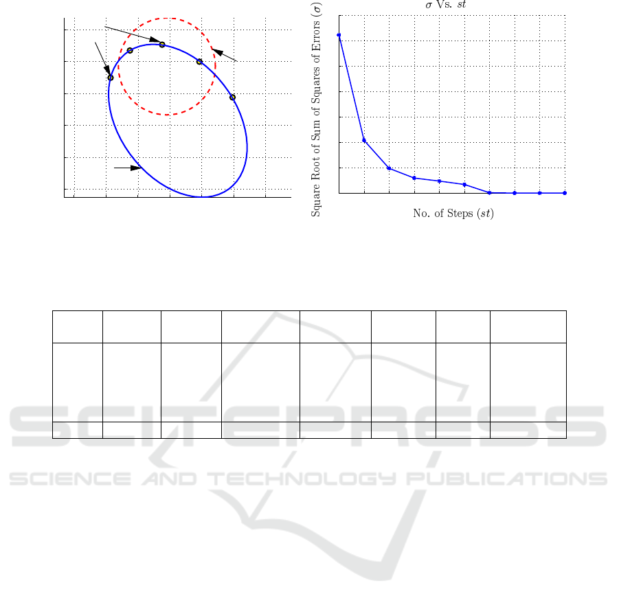
As the proposed general conic fitting method does not
require much precision in the initialization, the cir-
cle shown above can very conveniently be used as
the initial guess. An example of a conic fitting, with
this initialization is shown in figure 4(a), along with
the square root of the squared sum of orthogonal dis-
tances, from the points to the estimated conic at each
step of the optimization in figure 4(b).
4 EXPERIMENTAL RESULTS
First, we evaluated the performance of the algorithm
for points on randomly generated conics. For this ex-
periment, 1000 random conics were generated, and 5,
10, 15, 20 and 25 points on these conics were selected
randomly. Then, the proposed general conic fitting
algorithm was run on the points. The type of conic
was not restricted in any way, except that a check was
done for imaginary conics, and in a situation where
one was generated, it was discarded, and another ran-
dom conic generated in its place. Table 1 shows the
results of the fitting, where all the values are averaged
over the 1000 random conics. σ is the square root
of the mean squared orthogonal distance, while σ
n
is
the same error normalized over the number of points,
calculated for the sake of comparison where different
numbers of points are involved in the fitting.
Table 1 shows that the mean error per point σ
n
on
average (for all 5000 cases) is less than 0.3 pixels.
Furthermore, the results indicate that the number of
fits that have an error less than 0.001, 0.01, 0.1, and
1 are 65.72%, 80.88%, 92.82%, and 96.74% respec-
tively. The average number of iterations to conver-
gence is approximately 16 steps. For a general conic
fitting algorithm, these results are very accurate, and
the speed of convergence is also acceptable ( see (Ahn
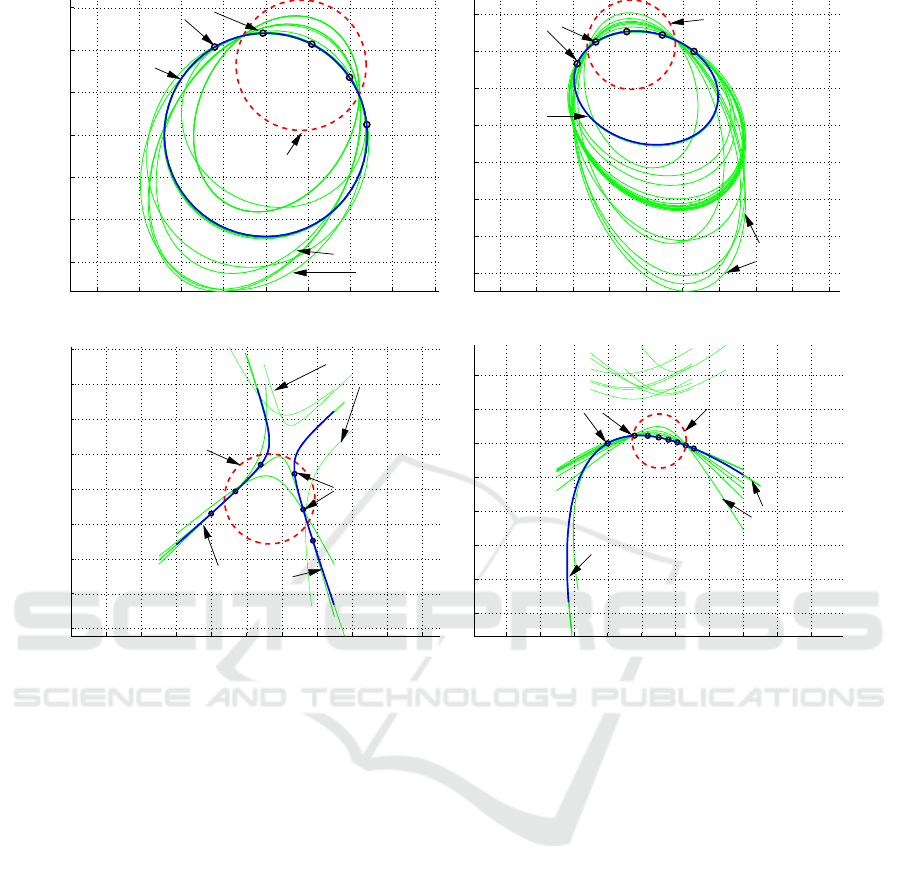
et al., 2001)). Figure 5 shows how the proposed algo-
rithm performed on some points on random conics of
different types.
Next, we compared the performance of the pro-
posed conic fitting algorithm with other orthogonal
distance fitting methods. To this end, first, we com-
pare the time complexities of existing algorithms, iter-
ative and non-iterative in their method of determining
the orthogonal distance. Then, we focus on the per-
formance of the proposed algorithm with others that
calculate the orthogonal distance directly (but using
conic specific information).
The general orthogonal distance fitting algorithm
introduced in (Boggs et al., 1987) determines the
model parameters and the orthogonal points simulta-
neously and has a time/space complexity of O(n
2
),
while (Helfrich and Zwick, 1993) present a nested it-
eration scheme with a time complexity of O(n). The
general nested iterative method discussed in (Ahn,
2004) has similar time/space complexities. The pro-
posed algorithm, also has time and memory usage
proportional to the number of data points O(n), but
removes the nested iteration scheme of (Ahn, 2004)
by calculating the orthogonal distance non-iteratively.
The type specific direct fitting methods such as (Ahn
et al., 2001), (Gander et al., 1994), and (Spath, 1995)
also have the same time complexity and require a non-
VISAPP 2009 - International Conference on Computer Vision Theory and Applications
142
−15 −10 −5 0 5 10 15
0
5
10
15
20
25
Points
Data
Fitted
Conic
Initial
Conic
(a) Initial and Fitted Conics
1 2 3 4 5 6 7 8 9 10
0
20
40
60
80
100
120
140
(b) Error at each Step of the Optimization
Figure 4: Fitting of a Conic.
Table 1: Results for the Fitting of Random Conics.
Points Avg. σ Avg. σ
n
σ
n
< 0.001 σ
n
< 0.01 σ
n
< 0.1 σ
n
< 1 Avg. Steps
(pixels) (pixels) (%) (%) (%) (%)
5 1.2505 0.2501 78.1 85.5 92.4 97.4 17.29
10 1.7653 0.1765 64.6 81.3 91.6 96.2 16.33
15 4.5601 0.3040 60.6 79.3 92.5 95.9 17.11
20 4.7040 0.2352 65.0 81.0 95.3 97.5 15.26
25 7.7385 0.3095 60.3 77.3 92.3 96.7 14.60
Avg. N/A 0.2551 65.72 80.88 92.82 96.74 16.12
nested iteration for the fitting.
In light of the similarity in terms of the type of it-
eration (nested or not) and time/space complexity, the
performance of the proposed algorithm can be evalu-
ated against other direct fitting methods (Ahn et al.,
2001; Gander et al., 1994; Spath, 1995). With re-
spect to the others, the proposed method has a clear
advantage in that, it has a time/space complexity of
O(n) and that it uses a non-nested iterative scheme. It
should also be noted that, in most of these methods,
accurate initial guesses are required for good perfor-
mance. Therefore, algebraic (or in some cases, or-
thogonal) fitting is required to provide the initializa-
tion, whereas the proposed algorithm is more robust
and requires only a loose initialization in the form of
the RMS circle, irrespective of the type of conic the
data resembles, as shown in the previous experiment.
Table 2 summarizes the results of the compari-
son of the direct conic fitting algorithms with respect
to the data sets in (Gander et al., 1994) and (Spath,
1995). The data sets are for different conic types, and
therefore, only the relevant algorithms were run on
specific data sets. For example, the data sets provided
for ellipse fitting were used only on ellipse specific al-
gorithms. On the contrary, as the proposed algorithm
is type independent, it was run on all data sets.
Further, to make the comparison more consistent,
the results of the same algorithm, which uses differ-
ent initializations, were averaged. For example, in the
circle fitting of (Ahn et al., 2001), two initializations
were used: the RMS circle, and an algebraically fit-
ted circle. The results in table 2 shows the average
performance of the two. This is done in an attempt
to make the comparison more independent of the type
of initialization used. For details on individual per-
formance on various data sets with different initializa-
tions, refer to (Wijewickrema et al., 2006) and (Ahn
et al., 2001).
Note that the error σ
avg
is the square root of the
mean squared orthogonal distance to the fitted conic,
and k ∆p k
avg
is the average of the norm of the pa-
rameter update vector. As seen from the results, even
dedicated fitting methods do not achieve the accuracy
of the general algorithm proposed here, which scores
the lowest value of σ
avg
= 0.8813, over all others. The
number of iteration steps, although higher than that of
the others, is acceptable considering the rough initial-
ization and type independent nature of the algorithm.
Therefore, from the results, it is seen that the pro-
posed orthogonal distance fitting method performs
A NOVEL APPROACH TO ORTHOGONAL DISTANCE LEAST SQUARES FITTING OF GENERAL CONICS
143
0 5 10 15 20 25 30 35 40
−5
0
5
10
15
20
25
Fitted Conic
PointsData
Initial Conic
Intermediate
Steps
(a) Circle
−20 −10 0 10 20 30 40 50 60 70
−40
−30
−20
−10
0
10
20
30
Data Points
Intermediate
Steps
Initial Conic
Fitted
Conic
(b) Ellipse
−40 −30 −20 −10 0 10 20 30 40 50 60
−40
−30
−20
−10
0
10
20
30
40
Steps
Intermediate
Data Points
Initial
Conic
Fitted Conic
(c) Hyperbola
−10 0 10 20 30 40 50 60 70 80
−40
−30
−20
−10
0
10
20
30
Intermediate
Steps
Initial ConicData Points
Fitted Conic
(d) Parabola
Figure 5: Fitting of Different Types of Conics using the Proposed Algorithm.
exceptionally well on noisy as well as noiseless data.
However, it should be noted that, for relatively
high levels of noise, the algorithm sometimes con-
verges to local minima, as is the case with algorithms
of its kind. To avoid this, a better initialization such as
an algebraic fit can be used with the same algorithm.
5 CONCLUSIONS
In this paper, we have introduced a novel algorithm
of orthogonal distance least squares fitting for gen-
eral conics. We have then illustrated the accuracy
and robustness of the algorithm by testing it on both
noiseless and noisy data and comparing with other di-
rect conic fitting methods. The main strength of the
method is the simplicity of calculation and the fact
that it can be used on any type of conic. The ad-
vantages of this proposed method as opposed to the
existing methods are as follows:
1. Conic (type) specific information is not required
2. Achieves higher accuracy with a similar (or
slightly higher) number of iterations
3. Simpler calculation of the orthogonal point and
the Jacobian Matrix
4. No prior fitting (algebraic or geometric) is re-
quired to obtain initial values (the same simple
procedure can be used to obtain the initial values
when fitting any conic)
Hence, we conclude that the above discussed al-
gorithm is powerful and robust (in terms of requiring
only a loose initialization in cases of relatively low
noise) and in its simplicity, is quite suitable to be used
in general conic fitting.
REFERENCES
Ahn, S. J. (2004). Least Squares Orthogonal Distance Fit-
ting of Curves and Surfaces in Space. Lecture Notes
in Computer Science, Vol.3151, Springer.
Ahn, S. J., Rauh, W., and Warnecke, H. J. (2001).
Least squares orthogonal distance fitting of circle,
VISAPP 2009 - International Conference on Computer Vision Theory and Applications
144

Table 2: Comparison of Direct Orthogonal Distance Fitting Algorithms.
Algorithm Type Avg. Steps k ∆p k
avg
Error σ
avg
(pixels)
Proposed General 13.1 4.3 ×10
−6
0.8813
Ahn Circle 8.5 4.5 ×10
−6
1.1080
Gander Circle 11 2.1 ×10
−6
1.1080
Sp¨ath Circle 116 1.0 ×10
−4
1.1080
Ahn Ellipse 16.5 4.03 ×10
−6
1.2581
Gander Ellipse 71 1.0 × 10
−6
1.1719
Sp¨ath Ellipse 30 1.0 ×10
−4
1.4306
Ahn Hyperbola 6.4 3 × 10
−6
0.8899
Sp¨ath Hyperbola 100 1.0 × 10
−4
1.2532
Ahn Parabola 11.7 5.9 × 10
−6
1.9263
Sp¨ath Parabola 53.5 5.3 × 10
−5
2.1854
sphere, hyperbola and parabola. Pattern Recognition,
34:2283–2303.
Boggs, P. T., Byrd, R. H., and Schnabel, R. B. (1987). A
stable and efficient algorithm for nonlinear orthogonal
distance regression. SIAM Journal of Scientific and
Statistical Computing, 8(6):1052–1078.
Chaudhuri, B. B. and Samanta, G. P. (1991). Elliptic fit
of objects in two and three dimensions by moment
of inertia optimization. Pattern Recognition Letters,
12(1):1–7.
Faber, P. and Fisher, R. B. (2001). Euclidean fitting revis-
ited. Lecture Notes in Computer Science, 2059:165–
172.
Fitzgibbon, A. W. and Fisher, R. B. (1995). A buyer’s guide
to conic fitting. In British Machine Vision Conference,
pages 513–522, Birmingham , UK.
Gander, W., Golub, G. H., and Strebel, R. (1994). Least-
squares fitting of circles and ellipses. BIT, 34:558–
578.
Gauss, C. F. (1963). Theory of the motion of heavenly
bodies moving about the sun in conic sections (theo-
ria motus corporum coelestium in sectionibus conicis
solem ambientium). First published in 1809, Transla-
tion by C. H. Davis. New York: Dover.
Hartley, R. and Zisserman, A. (2003). Multiple View Geom-
etry in Computer Vision. Cambridge University Press.
Helfrich, H.-P. and Zwick, D. (1993). A trust region method
for implicit orthogonal distance regression. Numerical
Algorithms, 5:535–545.
Hough, P. V. C. (1962). Methods and means for recognizing
complex patterns. US Patent 3 069 654.
Ma, Y., Soatto, S., Kosecka, J., and Sastry, S. S. (2004). An
Invitation to 3D Vision. Springer.
Miller, J. R. (1988). Analysis of Quadric Surface based
Solid Models. IEEE Computer Graphics and Appli-
cations, 8(1):28–42.
Press, W. H., Flannery, B. P., Teukolsky, S. A., and Vetter-
ling, W. T. (1992). Numerical Recipes in C. Cam-
bridge University Press, 2nd Edition.
Semple, J. G. and Kneebone, G. T. (1956). Algebraic Pro-
jective Geometry. Oxford University Press.
Spath, H. (1995). Orthogonal squared distance fitting with
parabolas. In G. Alefeld, J. Herzberger (Eds.), Pro-
ceedings of the IMACS-GAMM International Sympo-
sium on Numerical Methods and Error-Bounds, Uni-
versity of Oldenburg, pages 261–269.
Taubin, G. (1991). Estimation of planar curves, surfaces and
nonplanar space curves defined by implicit equations,
with applications to edge and range image segmenta-
tion. IEEE Transactions on Pattern Analysis and Ma-
chine Intelligence, 13(11):1115–1138.
Wijewickrema, S. N. R., Papli
´
nski, A. P., and Esson, C. E.
(2006). Orthogonal distance fitting revisited. Techni-
cal Report 2006/205, Clayton School of Information
Technology, Monash University, Melbourne, Aus-
tralia.
Young, J. W. (1930). Projective Geometry. The Mathemat-
ical Association of America.
A NOVEL APPROACH TO ORTHOGONAL DISTANCE LEAST SQUARES FITTING OF GENERAL CONICS
145
