CLASSIFIERS SENSITIVITY FOR BOUNDARY CASE TESTING

SET IN THE FACE RECOGNITION ALGORITHM BASED ON

THE ACTIVE SHAPE MODEL

Andrzej Florek and Maciej Król

Institute of Control and Information Engineering, Automatic Control and Robotics Division

Poznan University of Technology, str. Piotrowo 3A, 60-965 Poznań, Poland

Keywords: Face recognition, Active Shape Model, Principal Component Analysis, Linear Discriminant Analysis,

Support Vector Machine and Classification.

Abstract: In this paper, experimental results from the face contour classification tests are shown. The presented

approach is dedicated to a face recognition algorithm based on the Active Shape Model method. The results

were obtained from experiments carried out on the set of 3300 images taken from 100 persons.

Automatically fitted contours (as 194 ordered face contour points vector, where the contour consisted of

eight components) were classified by Nearest Neighbourhood Classifier and Support Vector Machines

classifier, after feature space decomposition, carried out by the Linear Discriminant Analysis method.

Feature subspace size reduction and classification sensitivity analysis for boundary case testing set are

presented.

1 INTRODUCTION

In this paper, a discussion concerning the choice of

a classifier for the face recognition algorithm is

presented. We investigate how the classification

sensitivity coefficient is influenced by: the feature

vector size, the size of the Principal Component

Analysis (PCA) used for contours validation

procedure, the size of the Linear Discriminant

Analysis (LDA), number of classes and boundary

case testing set. The presented algorithm for face

classification is based on the Active Shape Model

method (ASM) introduced by Cootes (Cootes and

Taylor, 2001), which is a modification of the Active

Contour Model method (ACM), i.e. a snake-based

approach to extracting face contour from an image

(Kass and Witkin, 1988). The ASM is a two-stage

algorithm and it is based on a shape notation, which

is defined as an ordered set of points. First, a Point

Distribution Model (PDM) is produced, which will

be used for validation of a contour shape. Next,

a Local Grey Level Model (LGLM) is generated for

interactive fitting of the contour points to the local

image context. This method is still in progress,

where modifications consist of initial contour choice

and the new fitting methods (Zao and Li, 2004),

(Zuo and de With, 2004). The ASM has been

successfully used to extract the facial features of

a face image under frontal view. However, its

performance degrades when the concerned face is

under perspective variations. For this reason,

a modified shape model was proposed by Wan and

Lam (Wan and Lam, 2005). It can adapt face images

from different orientations or facial expressions

and

represents a face more flexibly.

To obtain PDM and LGLM models, the desirable

contour localization on an image of a person has to

be known. Thus, placing contours onto images

(chosen to create a learning set) has to be performed

and this may be done manually or automatically.

Arrangement of proper learning set is usually the

most important problem of a good classifier choice.

A standard approach to classification consists of

determining an affiliation of a sample to a class

represented by its model. To construct a model of

a person, a set of images has to be produced. These

images have to be divided into learning and testing

sets, for example by simple sampling or multiple

sampling with replacement. The classification

improvement should be achieved by removing the

identified outliers from a training set. Generally, the

database is built under surveillance of specialists and

281

Florek A. and KrÃ¸sl M.

CLASSIFIERS SENSITIVITY FOR BOUNDARY CASE TESTING SET IN THE FACE RECOGNITION ALGORITHM BASED ON THE ACTIVE SHAPE MODEL.

DOI: 10.5220/0001772902810287

In Proceedings of the Fourth International Conference on Computer Vision Theory and Applications (VISIGRAPP 2009), page

ISBN: 978-989-8111-69-2

under determined conditions (distance, light,

position, etc.). In practical vision system, the picture

of a person (sample) is taken without this

surveillance and allows the person a freedom of pose

and gesture. Thus, the classification efficiency is in

practice lower than it was anticipated. This problem

can occur in the situation, when we want to verify if

a person from an accidental image is not wanted. In

the presented paper, we propose another testing set,

which is obtained from images of faces in extreme

positions

under different perspective variations and

facial expressions than in the conventional learning

set (boundary cases).

2 CONTOURS

The shape in the ASM method is represented as an

ordered set of control points placed on contours

describing face elements and it is given by the

following vector

x = ( x

, y

, x

, y

,..., x

, y

)

, (1)

where x

and y

are coordinates of contour control

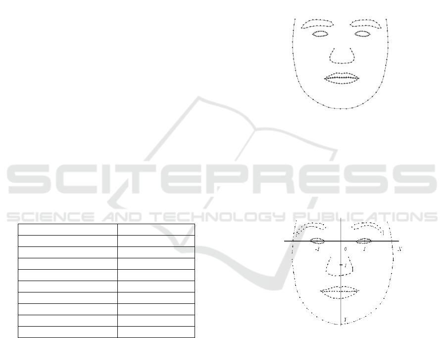
points. In the considered case, for eight chosen

components of face contours, n = 194 points have

been determined (Fig. 1 and Tab.1) and this implies

388-dimensional shape space.

Table 1: Face contours.

Contou

Number of points

Face outline FO 41

Mouth outer MO 28

Mouth inner MI

Right eyelid REL 20

Left eyelid LEL 20

Right eyebrow REB 20

Left eyebrow LEB 20

Nose outline NO 17

TOTAL

194

2.1 Extracting and Calculation of

Contours

To obtain normalized learning contours, the initial

contour (template – Fig. 1) is placed on the image.

Next, it is manually fitted to the correct place that

the operator regards as the best localization for the

contour points. Subsequently, the derived contours

are normalized. Scale coefficient and rotation of

contour result from the calculated coordinates of eye

centres (pupils). Pupil coordinates are calculated

from coordinated contour points located in the eyelid

corners. Pupil coordinates determine X-axis; points

(-1, 0), (1, 0) are located on right and left pupil,

respectively. The symmetrical of this section

determines Y-axis and the middle of coordinate

system. Next, the contour points are projected on

a normalized coordinate system. The normalized

contour has to be uniformly sampled (manually

extracted contours do not have uniform distances

between the adjacent contour control points). The

normalized and uniformly sampled contours are

presented in Fig. 2.

Figure 1: Template contour.

During the normalization procedure, points are

ordered in a defined sequence, according to the

feature vector definition (1). In the presented

approach, the height standardization of face and

nose outlines has not been applied.

Figure 2: Normalized manually fitted contour.

3 EXPERIMENT

In order to select classifiers for the ASM face

recognition algorithm, an experiment consisting of

examining a set of face images was undertaken.

Colour images of 2048 × 1536 pixels were used. For

100 persons (100 classes) the following images were

taken (Fig. 11 and 12):

H – sequence of 30 frames for horizontal head

rotation from the right to the left half-profile;

VISAPP 2009 - International Conference on Computer Vision Theory and Applications

282

V – sequence of 20 frames for vertical face rotation

from slightly risen to hang down head

position;

D – frames for different head positions and facial

expressions

(boundary cases).

The contours were manually positioned on 11

central succeeding images (frames) from H and V

sequences. In presented experiment, 2200 contours

were used as the manual learning set (LSM) for the

ASM algorithm (to determine PDM and LGLM

models). Next, the ASM algorithm was performed to

generate automatic contours for images from H and

V sequences and additionally from D-sequence.

3.1 Set Definitions

The normalized automatic contours were divided

into the following sets (see Fig. 11 and 12):

 LSA – automatic learning set, 2200 contours,

100 classes, 22 contours for each class (11

central from H sequence and 11 central from V

sequence);

 A – learning or testing set, 1100 contours, 100

classes, 11 contours for each class, even frames

subset of LSA;

 B – learning or testing set, 1100 contours, 100

classes, 11 contours for each class, odd frames

subset of LSA;

 C100 – testing set, 1100 automatic contours,

100 classes, 11 contours for each person from

H, V (boundary case in relation to LSA) and D.

The boundary case set C100 is almost a “regular

and balanced set”, i.e. consists of 4 contours from

both H and V sequences, (out of 11 central images)

and of 3 contours from D sequence. In the goal to

examine influence of number of classes on

classification sensitivity coefficient, the set C100

was also divided to subsets Cnc, where nc is the

number of classes, i.e. two C50, three C33, four C25

and five C20. From analogical reasons, the learning

set LSA was divided in the equivalent manner too.

Both A and B sets were used as learning or

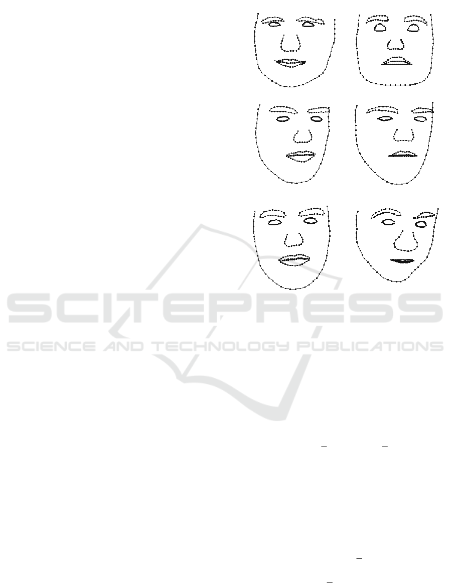
testing sets alternatively. The normalized contours

from testing set C100 were slightly different for the

same person than those from learning sets (Fig. 3).

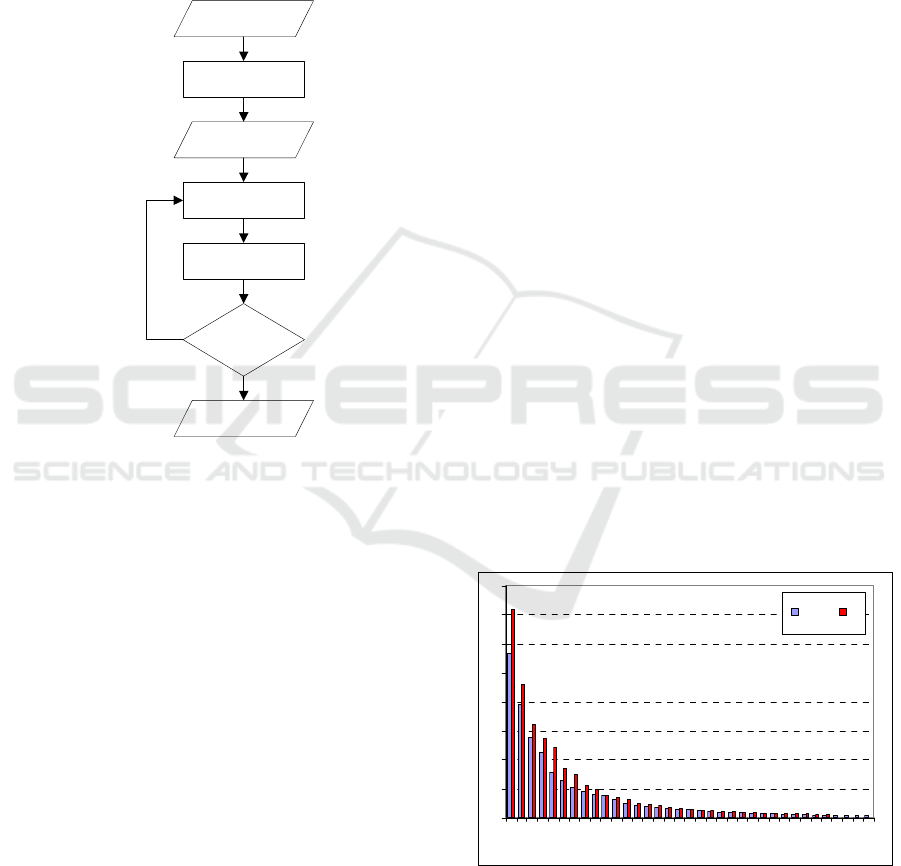
3.2 Contour fitting

The algorithm of contour fitting utilizes the ASM

method (Fig. 4). Firstly, Gaussian pyramid for input

image is generated. The initial contour shape is

placed at the coarsest level of the pyramid.

Secondly, the initial contour is initialised by placing

the mean face shape model (calculated from learning

Figure 3: Normalized contours: manual contours from the

learning set LSM (left column); automatic contours from

the testing set C100 (right column).

set LSM, see Fig. 1) at the position of localized face.

Two steps of the ASM algorithm (LGLM and PDM

– Fig. 4) are executed in a loop. The LGLM step

locates salient features of image along the normal

direction of contour control points. Each contour

point (x

, y

) is shifted along the normal to the best

matching position (x

, y

). The matching error is

defined as minimal Mahalonobis distance d

()()

iiji

iijij

δδδδ

−−=

−1

(2)

from current LGL profile

to mean profile

⎯δ

for

a given contour control point. The mean

⎯δ

and

covariance C

are computed from local grey level

around manual contours control points (LSM) taken

from learning set of images.

In the PDM step, the shape is filtered with

forward (3) and inverse (4) transformations

()

xxb

−= P

(3)

bxx P+≈

(4)

to and from the subspace reduced by the PCA. The

transformation matrix P is selected as the first p-

CLASSIFIERS SENSITIVITY FOR BOUNDARY CASE TESTING SET IN THE FACE RECOGNITION ALGORITHM

BASED ON THE ACTIVE SHAPE MODEL

283

eigenvectors (p first PCs) of covariance matrix of

contours from learning set. In the presented paper,

value p=45 were used at 98,8% total variance ratio.

The choice of this size is very important because it

affects classification efficiency for applied classifier

(this will be discussed later in this paper). The

iteration ends when shapes stop changing

significantly and computation is repeated for finer

level of image pyramid until the last level is reached.

Figure 4: ASM algorithm diagram.

3.3 Classifiers

Three classification methods were tested. The first

classifier was the Nearest Neighbourhood Classifier

(NNC) in reduced to k-size feature shape subspace,

derived from LDA/k decomposition. As a metric,

Euclidean distance to a model of class in subspaces

for different size k was used (subspaces are not

orthogonal). The second method was taken as the

SVM method using a Radial Basis Function as

kernel and one-to-one voting system with a tie-

breaking algorithm. In the presented approach, SVM

classifiers were applied in full feature space and in

its k-subspaces (the third method), obtained after the

LDA/k decomposition in the feature space. As

sensitivity measure of classifiers (recognition rate)

the coefficient TP/(TP+FN) in percent was chosen,

where TP and FN are numbers of True Positive (the

person correctly recognized) and False Negative (the

person not properly recognized) classifications.

Classification methods are denoted as:

 LDA/k – Euclidean distance in k-size

feature space reduced after Linear

Discriminant Analysis;

 SVM – SVM classifier in full 388-

dimentional feature space;

 LDA/k & SVM – SVM classifier in LDA

subspace reduced to k-size.

3.4 Choice of PCA Size for PDM

Validation

Determining the dimensionality of the PCA

subspace, i.e. the number of PCs to represent face

patterns (contours), is an intricate problem. It is

usually a trade

-off between estimation accuracy and

computational efficiency (Motulsky, 1997).

Calculated eigenvalues and cumulative variances are

presented in Fig. 5 and 6.

The reduction of the feature vector space to

around the first p=30 PCs seems to be reasonable

(97% of total data variance). Classification results

for learning set LSA (average from tests where A and

B sets were used as learning or testing sets

alternatively) are presented in Fig. 7 and confirm the

choice of first 30 PCs. However, results for

boundary case testing set C suggest that the

dimension size p= 45 (98,8% of total variance) will

be better for LDA classifier. Small vector size in the

PDM validation stage in the ASM algorithm unifies

contours and smoothes between-class differences.

Large vector size causes relaxation of contour and

reduces noise resistance. For the PDM validation

procedure in performed ASM algorithm, vector of

the first 45 PCs was chosen.

Figure 5: Eigenvalues in the PCA decomposition.

face image

face detection

LGL localization

PDM validation

shape

converged?

face shape

Yes

initial shape

1 6 11 16 21 26 31

Eigenvalue index p

LSA C

VISAPP 2009 - International Conference on Computer Vision Theory and Applications

284

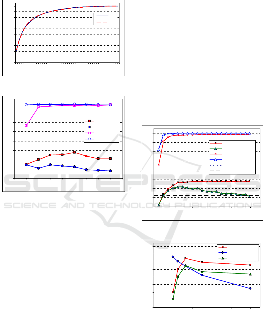
Figure 6: Cumulative variance in the PCA decomposition.

Figure 7: Classification sensitivity for LSA and C100 sets.

3.5 Results and Discussion

The SVM method is commonly used for

classification. As we can see in Fig. 7, this method is

good for testing samples similar to those from

learning set (i.e. when they are close with respect to

the face position and gestures). Classification

efficiency obtained from LSA set was equal (or very

close) to 100%. Experimental results demonstrate

good property of SVM classifier, however this is the

situation where the learning and testing sets were

regular subsets of larger learning set LSA. For the set

C as the testing set, the LDA classifier was much

better than the SVM classifier in full-dimensional

feature space. This suggests that the LDA method is

more resistant to diversity of a testing set, because

the space transformation function is found in order

to maximize the ratio of between-class variance to

within-class variance. In subsequent tests we

investigated influence of the proposed LDA

decomposition on amelioration of classification

sensitivity for boundary case set. Results are

presented in Fig. 8 We can observe that the LDA

decomposition of order higher than PDM model is

not necessary for the LDA classifier (for large

feature vector size the maximal LDA size is equal to

(nc-1), where nc is the number of classes). On the

other hand, LDA feature vector size reduction can

ameliorate sensibility of SVM classifier (denoted as

LDA /k & SVM classifier). Influence of class

number on classification sensitivity is presented in

Fig. 9 and 10. Results for nc classes were averaged,

for example for nc=25, testing C100 and learning

LSA sets were divided into 4 separate pairs of

subsets and partial classifications results were

averaged. Results demonstrate that for small number

of classes in relation to the size of feature vector (1),

the SVM classifier is much better then classifier

based on LDA decomposition. This low LDA

classification sensitivity mainly comes from ill-

conditioned between-classes scatter matrix.

Figure 8: Classification sensitivity for LSA and C100 sets.

Figure 9: Classification sensitivity for testing sets Cnc.

10%

20%

30%

40%

50%

60%

70%

80%

90%

100%

1 6 11 16 21 26 31 36 41 46

Number of eigenvalues p

LSA

20%

30%

40%

50%

60%

70%

80%

90%

100%

20 25 30 35 40 45 50 55 60 65

PCA validation size p

LDA /99 {C100}

SVM {C100}

LDA /99 {LSA}

SVM {LSA}

20%

30%

40%

50%

60%

70%

80%

90%

100%

020406080100

imension k of LDA subspace

LDA /k {C100}

LDA /k & SVM {C100}

LDA /k {LSA}

LDA /k & SVM {LSA}

SVM lev el {LSA}

SVM lev el {C100}

20%

25%

30%

35%

40%

45%

50%

55%

60%

020406080100

Number of classes nc

LDA /(nc-1)

SVM

(LDA /k & SVM) max

CLASSIFIERS SENSITIVITY FOR BOUNDARY CASE TESTING SET IN THE FACE RECOGNITION ALGORITHM

BASED ON THE ACTIVE SHAPE MODEL

285

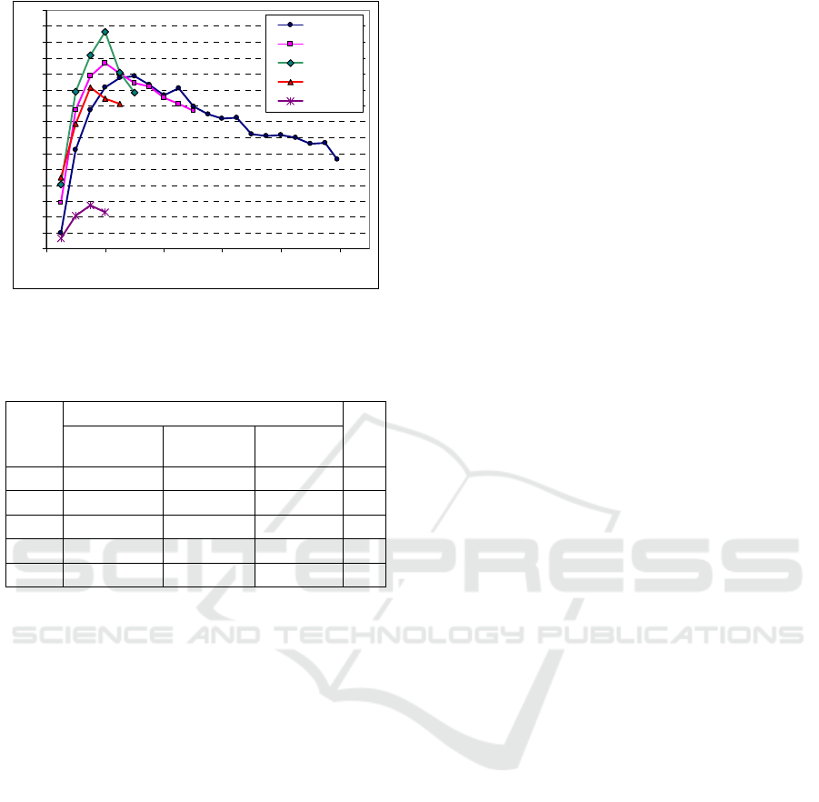
Figure 10: LDA /k & SVM classification sensitivity for

testing sets Cnc.

Table 2: LDA /k & SVM classification sensitivity for

testing sets Cnc.

4 SUMMARY

The ASM produces reasonably good face contours

for our boundary case testing set (Fig. 11 and 12). It

is able to handle face images with glasses, beard and

long hair. We have found out that ASM has

problems with fitting contours to images with non-

frontal face orientation.

It is caused by linear nature of Point Distribution

Model (PDM), which utilizes the PCA validation

procedure (Fig. 4). The PDM validation procedure

filters contours according to the first PCs directions

in the learning set (3 and 4). This is a significant

disadvantage of ASM algorithm which leads to

blurring between-classes differences. Authors in

(Etamad and Chellapa, 1997) underline that the

LDA of faces provides us with a small set of

features that carry the most relevant information for

classification purposes. For medium-sized databases

of human faces, good classification accuracy is

achieved using very low-dimensional feature

vectors.

In this paper, an experiment consisting of

application of boundary case testing set for tuning

ASM parameters and for amelioration of SVM

classifier sensitivity was presented. It has turned out

that same size reduction (according to LDA results)

improves the sensitivity of SVM classifier (Fig. 8

and 10). The optimal size of reduced LDA-subspace

is lower than PDM validation vector size and much

lower than the number of classes k‹‹(nc-1),

investigated in the test (Fig. 10 and Tab. 2). This

condition for size k improves attenuation of

disturbances. Those disturbances are understood as

differences between learning and testing sets

(extreme face positions

under different perspective

variations and facial expressions). Generally, for

large number of classes, the LDA classifier is better

than SVM, but for small number of classes we

observe inverse situation (Fig. 9).

It is desirable to examine influence of other

contour normalisation procedures. In presented

experiments, the height standardisation of face and

nose outlines has not been applied. Other

normalisation procedures, such as application of

initial contour determined by calculated face

position (Ge and Yang, 2005) and identified face

gestures and head position (Wan and Lam, 2005)

will be verified in the future research.

REFERENCES

Cootes, T. and Taylor, C., (2001). Statistical models of

appearance for computer vision, Technical report,

University of Manchester, Wolfson Image Analysis

Unit, Imaging Science and Biomedical Engineering.

Etemad K., Chellappa R. (1997), Discriminant analysis

for recognition of human face images, Springer Berlin

/ Heidelberg.

Ge, X., Yang, J., Zheng, Z., Li, F., (2006). Multi-view

based face chin contour extraction, Engineering

Applications of Artificial Intelligence, vol.19, pp. 545-

555.

Kass, M., Witkin, A., Terzopoulos, D., (1988). Snakes:

Active contour models, International Journal of

Computer Vision, 1 (4), pp. 321-331.

Motulsky, H., (1997). Detecting outliers, GraphPad

Insight, issue number 14, Winter 1997.

Wan, K.W., Lam. K.M., Ng, K.C., (2005). An accurate

active shape model for facial feature extraction,

Pattern Recognition Letters, vol. 26 , Issue 15, pp.

2409-2423.

Zhao, M., Li, S. Z., Chen, Ch., Bu, J., (2004). Shape

evaluation for weighted active shape models,

Proceedings of the Asian Conference on Computer

Vision, pp 1074-1079.

Zuo, F. and de With, P. H N., (2004). Fast facial feature

extraction using a deformable shape model with Haar-

wavelet based local texture attributes, Proceedings of

ICIP’04, vol. 3, pp. 1425-14

20%

22%

24%

26%

28%

30%

32%

34%

36%

38%

40%

42%

44%

46%

48%

50%

0 20406080100

Dimension k of LDA subspace

1 x {C100}

2 x {C50}

3 x {C33}

4 x {C25}

5 x {C20}

No. of

classe

s nc

Classification sensitivity in %

max

LDA /(nc-1) SVM

(LDA /k &

SVM)

max

20 29,9 53,2 25,5 15

25 44,9 50,1 40,3 15

33 52,1 46,9 47,3 20

50 49,5 40,9 43,4 20

100 47,6 32,3 41,7 30

VISAPP 2009 - International Conference on Computer Vision Theory and Applications

286

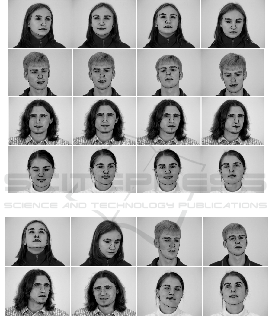
Figure 11: Images and contours from learning set LSA fitted by the ASM algorithm.

Figure 12: Images and boundary case contours from testing set C100 fitted by the ASM algorithm.

CLASSIFIERS SENSITIVITY FOR BOUNDARY CASE TESTING SET IN THE FACE RECOGNITION ALGORITHM

BASED ON THE ACTIVE SHAPE MODEL

287