COMBINING TEXTURE SYNTHESIS AND DIFFUSION FOR IMAGE

INPAINTING

Aur´elie Bugeau

Image processing group, Barcelona Media, Barcelona, Spain

Marcelo Bertalm´ıo

Dept. de Tecnologies de la Informaci´o i les Comunicacions, Universitat Pompeu Fabra, Barcelona, Spain

Keywords:

Image inpainting, Texture synthesis, Structure, Diffusion, Image decomposition.

Abstract:

Image inpainting or image completion consists in ﬁlling in the missing data of an image in a visually plausible

way. Many works on this subject have been proposed these recent years. They can mainly be decomposed

into two groups: geometric methods and texture synthesis methods. Texture synthesis methods work best with

images containing only textures while geometric approaches are limited to smooth images containing strong

edges. In this paper, we ﬁrst present an extended state of the art. Then a new algorithm dedicated to both

types of images is introduced. The basic idea is to decompose the original image into a structure and a texture

image. Each of them is then ﬁlled in with some extensions of one of the best methods from the literature.

A comparison with some existing methods on different natural images shows the strength of the proposed

approach.

1 INTRODUCTION

The problem of image completion or image inpaint-

ing can be deﬁned as follows: given an image con-

taining missing regions (corresponding for example

to some objects one wants to remove), the comple-

tion consists in ﬁlling in these missing parts in such

a way that the reconstructed image looks natural (i.e.

visually plausible). Basically, given a corrupted im-

age I : Φ → R

(or eventually I : Φ → R in case of

grayscale images) and a mask M : Φ → {0, 1}, the

inpainting algorithm must ﬁll in the region Ω where

M(p) = 0 (here p is a pixel belonging to Φ).

This problem is for the moment far to be solved.

Indeed, natural images are complex and may contain

different textures, strong structures (edges), etc. Ex-

isting methods can be divided into two main groups:

”geometric” methods which allow to get regularized

contours but do not give some nice reconstruction of

textured areas and texture synthesis methods which

basically do the opposite. Before going any further,

we now brieﬂy review these two types of approaches.

1.1 “Geometric” Methods

This ﬁrst category of image completionmethods try to

ﬁll-in the missing regions of an image through a diffu-

sion process, by propagating the information known

on the boundary towards the interior of the holes.

Generally these methods consist in ﬁnding the global

minimum of an energy function, by converging to the

steady state of the corresponding Partial Differential

Equation (PDE) (section 1.1.1). As, most of the time,

a lot of iterations are needed before the convergence

can be reached, these methods are computationally

expensive. Therefore some algorithms propagating

the information from the boundary inwards without

ﬁnding the global minimum of an energy function

have also been proposed (see section 1.1.2).

1.1.1 PDE’s based Image Inpainting

The term of ”digital inpainting” was ﬁrst introduced

in (Bertalmio et al., 2000). In this paper, a third or-

der PDE, solved only inside Ω with proper bound-

ary conditions in δΩ, was proposed. Its purpose is

to propagate image Laplacians in the isophote (line

of constant intensity) directions. The edges recovered

Bugeau A. and BertalmÃ o M.

COMBINING TEXTURE SYNTHESIS AND DIFFUSION FOR IMAGE INPAINTING.

DOI: 10.5220/0001773900260033

In Proceedings of the Fourth International Conference on Computer Vision Theory and Applications (VISIGRAPP 2009), page

ISBN: 978-989-8111-69-2

with this approach are smooth and continuous at the

boundary of the hole. However, it can not deal with

texture and, whenever the area to be inpainted is too

big, the result exhibits a lot of blur and is not contrast

invariant. This work was partly inspired by the Image

Disocclusion algorithm of Masnou and Morel (Mas-

nou and Morel, 1998) (see also (Masnou, 2002), in

which (an approximation of) the Elastica functional

was minimized inside the image gap. In (Ballester

et al., 2001) the Elastica functional is relaxed and then

minimized with a system of two coupled PDE’s.

Many other PDEs dedicated to inpainting have

been proposed in the literature. Inspired by

(Bertalmio et al., 2000), the authors of (Chan et al.,

2001) proposed to minimize the total variation en-

ergy which corresponds to a second-order PDE. How-

ever, this PDE does not maintain the curvature. With

this second-order PDE the contours are joined with

straight isophotes, not necessarily smoothly contin-

ued from the mask boundary. Hence, it is only in-

tended for small gaps. In (Chan and Shen, 2001),

the previous method has been extended by adding

a term diffusing the curvature in the direction nor-

mal to the isophote. It then becomes a third-order

PDE but still creates visible corners due to its straight

line connections. This is because the principle of

good continuation (the human visual system com-

pletes missing curves with curves that are as short and

as smooth as possible) is not respected. As a conse-

quence, a fourth-order PDE was proposed in (Chan

et al., 2002). It is based on the Euler’s elastica (Mum-

ford, 1994). Unfortunately, in pratice, this method is

extremely computationally consuming since conver-

gence requires a high number of iterations.

All previous PDEs where based on curvature dif-

fusion. Other PDEs, also relying on the isophotes

as was (Bertalmio et al., 2000), exist. For example,

in (Bertalm´ıo, 2006), a third-order PDE complying

with the principle of good continuation was proposed.

While this PDE is the best third order PDE for image

inpainting, it still does not well permit to handle im-

ages containing textures and its high order makes it

computationally expensive.

Another PDE method dedicated to anisotropic

smoothing was developed in (Tschumperl´e, 2006).

This method is based on the observation that all previ-

ous PDEs locally smooth (or diffuse) the image along

one or several directions that are different at each

image point, the principal smoothing direction being

parallel to the isophotes. As shown in this paper, an-

other approach is to retrieve the geometry of the main

structures inside the gap and to apply anisotropic dif-

fusion following this geometry. The geometry can be

retrieved using a structure tensor ﬁeld and the direc-

tion of the smoothing comes from a second ﬁeld of

diffusion tensors.

1.1.2 Inpainting based on Coherence Transport

The global resolution of all the PDEs previously

presented is made iteratively, which makes these

methods very time consuming. A non iterative

method, based on coherence transport, was proposed

in (Bornemann and M¨arz, 2007). This algorithm re-

lies on (Telea, 2004), in which Telea introduced a fast

algorithm for image inpainting that calculates the im-

age values inside the masks by traversing these pixels

in just a single pass using the fast marching technique.

The mask is ﬁlled in a ﬁxed order, from its boundary

inwards, using weighted means of already calculated

image values.

The main principle of the algorithm from (Borne-

mann and M¨arz, 2007) is to deﬁne the weights such

that the image information is transported in the direc-

tion of the isophotes. The directions of the edges are

extracted using the eigenvalues of structure tensors.

1.2 Texture Synthesis Methods

Given a texture sample, the texture synthesis prob-

lem consists in synthesizing other samples from the

texture. The usual assumption is that the sample is

large enough to capture the stationarity of the texture.

There have been many works extending texture syn-

thesis to inpainting. We here only present two of the

major works in this domain.

In the seminal paper (Efros and Leung, 1999), the

authors have presented a simple yet effective non-

parametric texture synthesis method based on local

image patches. The texture is modelled as a MRF by

assuming that the probability distribution of bright-

ness values for one pixel given the brightness values

of its spatial neighbourhood is independent from the

rest of the image. The neighbourhoodis a square win-

dow around the pixel and its size is ﬁxed by hand. The

input of the algorithm is a set of model image patches

and the task is to select an appropriate patch to predict

the value of an unknown pixel. This is done by com-

puting a distance measure between the known neigh-

bourhood of an unknown pixel and each of the input

patches. The distance is a sum of squared differences

(SSD) metric.

The authors of (Criminisi et al., 2004) proposed an

extension of Efros and Leung’s method, with two im-

provements. The ﬁrst one concerns the order in which

the pixels are synthesized. Indeed, a system for as-

signing priorities is used (assigning priorities to the

pixels was also proposed in (Harrison, 2001)). The

priority order at a pixel is the product of a conﬁdence

COMBINING TEXTURE SYNTHESIS AND DIFFUSION FOR IMAGE INPAINTING

term, which measures the amount of reliable informa-

tion surrounding the pixel, and a data term, that en-

courages linear structures to be synthesized ﬁrst. The

second improvement is a speed-up process. Contrary

to the original method in (Efros and Leung, 1999),

when synthesizing a pixel, not only the value of this

pixel is inpainted in the output image (using the patch

that givesthe smallest distance metric), but all the pix-

els in its neighbourhood that have to be inpainted are

ﬁlled in.

1.3 Overview of the Paper

As already mentioned, none of the previously de-

scribed methods is well adapted for all type of images.

In this paper we will therefore combine diffusion and

texture synthesis for image inpainting. Such a combi-

nation has already been proposed in (Bertalmio et al.,

2003). In the current work, we propose an exten-

sion to this paper mainly using some of the meth-

ods mentioned in this introduction. After reviewing

the method of (Bertalmio et al., 2003) in section 2, a

new algorithm will be proposed in section 3. We end

the paper with some experimental results and compar-

isons with existing approaches.

2 COMBINING TEXTURE

SYNTHESIS WITH DIFFUSION

Both texture synthesis and diffusion have their own

advantages and drawbacks for image inpainting.

While diffusion gives blurred results it allows a con-

tinuity of the contours. Texture synthesis permits to

conserve the textures but usually fails at preserving

the edges and big structures. Therefore combining

these two main types of approaches seems judicious.

As proposed in (Sun et al., 2005), a user can interact

to ﬁrst specify important missing structures, where a

speciﬁc structure propagation technique is applied. A

texture synthesis approach is then used to ﬁll in the

rest of the image. Another algorithm compining both

types of approaches without requiring any user inter-

vention is (Bertalmio et al., 2003). It is based on the

decomposition of the original image into a “structure”

and a “texture” image.

2.1 Structure/Texture Decomposition

A solution to keep the advantages of diffusion and

texture synthesis is to separate the image into a texture

image and a structure image. The problem is then to

ﬁnd a structure image u containing only the big struc-

tures of the original image I and a texture image v

such that:

I = u+ v. (1)

A method directly dedicated to ﬁnding these two

images has been proposed in (Vese and Osher, 2003).

The problem consists in ﬁnding the structure image

that minimizes the energy:

F(u) =

|∇u| + λ

kvk

. (2)

The ﬁrst term of eq.(2) is a smoothness term

whose role is to removethe noise, and the second term

is a data ﬁdelity term. This equation tends to remove

the noise while preserving the important structures.

Unfortunately, in (Meyer, 2001), Meyer showed that

when using eq.(2), the texture image does not only

contain oscillations (corresponding to noise) but also

the brightness’ edges. In fact, the L

space is not ap-

propriate for modelling oscillatory patterns. He there-

fore suggested to use the Banach space. The authors

of (Vese and Osher, 2003) proposed an algorithm to

decompose the original image into a texture and a

structure image in that case. An example of such a de-

composition is shown in ﬁgure 1. Note how the struc-

ture image (second column) looks like a cartoon im-

age that only contains important structures while the

texture images (third columns) contains mainly small

edges and noise.

2.2 An Existing Combination Algorithm

An inpainting algorithm based on a structure/texture

image decomposition has been presented in

(Bertalmio et al., 2003). The idea is to ﬁrst de-

compose the original image into a structure image

and a texture image using the method of (Vese and

Osher, 2003) previously presented. The structure

image is reconstructed by the inpainting method of

(Bertalmio et al., 2000) and the second one by the

texture synthesis of (Efros and Leung, 1999). The

resulting two images are ﬁnally added to obtain to

ﬁnal reconstructed image. This method gives less

artefacts on the contours of the reconstructed objects

than simple texture synthesis but it blurs the ﬁlling

region. Furthermore it stays limited to small image

gaps.

3 COMBINING TEXTURE

SYNTHESIS WITH DIFFUSION:

A NEW ALGORITHM

In this section we present the new algorithm we pro-

pose for image inpainting. It is an extension of the

VISAPP 2009 - International Conference on Computer Vision Theory and Applications

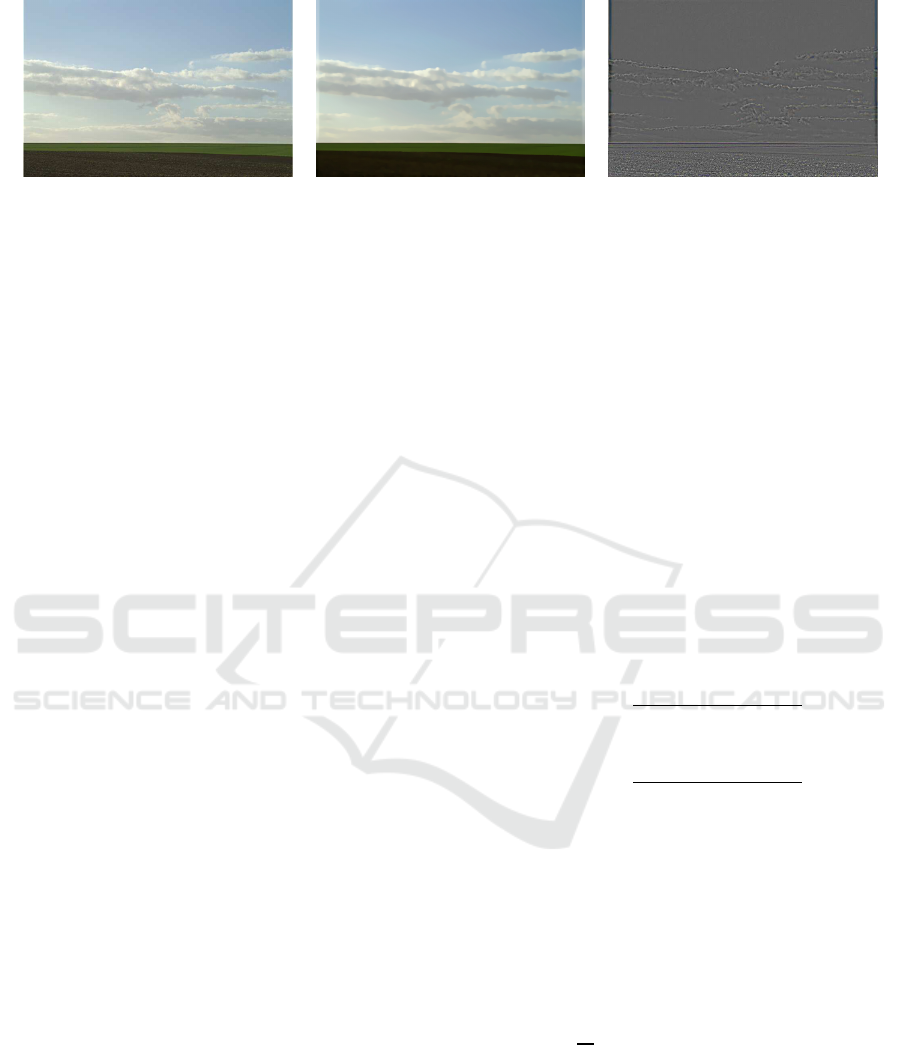
Figure 1: Result of the structure/texture decomposition algorithm from (Vese and Osher, 2003). The ﬁrst column shows the

original image, the second column the structure image, and ﬁnally the last one the texture image.

algorithm from (Bertalmio et al., 2003) presented in

the previous section. It is based on some improve-

ments to most of the steps involved. Therefore before

enumerating the whole algorithm, the presentation of

these improvements will be given.

3.1 Inpainting the Structure Image

In (Bertalmio et al., 2003) the so called “image in-

painting algorithm” from (Bertalmio et al., 2000) was

used to inpaint the structure image. This method

was brieﬂy presented in the introduction. It relies on

the resolution of a third order PDE that may cause

noticeable blur in the result image. Furthermore,

this third order PDE needs many iterations to con-

verge and is therefore computationally expensive. We

presented, in the same section, another PDE based

method (Tschumperl´e, 2006) that relies on a second

order PDE while rendering less blur. This method

gives very satisfactory results even after a small num-

ber of iterations. Therefore, the inpainting of the

structure image will here be done based on this al-

gorithm which we now describe in further details.

The main idea of geometric approaches is to dif-

fuse the colors along the isophotes which are con-

sidered to be the strong edges. The method from

(Tschumperl´e, 2006) follows the same scheme: the

direction of the main structures inside the gap is ﬁrst

computed and an anisotropic diffusion following this

geometry is then applied. A particularity here is that

the geometry is retrieved using structure tensor ﬁelds

(Weickert, 1998) and the geometry of the smoothing

comes from a second ﬁeld of diffusion tensors. For

a multi-valued image, the structure tensor is deﬁned,

for each pixel p, as:

J(p) =

∑

d=1

∇I

(p)∇I

(p), (3)

where ∇I

denotes the gradient image for the d

(color) channel. This tensor is a 2x2 symmetric and

semi-positive matrix. Its eigenvalues are positive and

can be ordered as: 0 ≤ λ

−

(p) ≤ λ

(p). The cor-

responding eigenvectors are denoted as θ

−

(p) and

(p). These eigenvectors represent two orthogonal

directions directed along the local maximum (gener-

ally normal) and minimum (generally tangent) vari-

ations of image intensities at pixel p. The eigenval-

ues then measure the effective variations (strength of

an edge) of the image intensities along these vectors.

The local smoothing geometry that should derive the

diffusion process is given by the ﬁeld of diffusion

tensors (Weickert, 1998; Tschumperle and Deriche,

2005). This ﬁeld, denoted as T, depends on the local

geometry and is deﬁned, for each pixel p, as:

T(p) = f

−

(p)θ

−

(p)θ

−

(p)

+ f

(p)θ

(p)

. (4)

The functions f

−

and f

set the strengths of

the desired smoothing along the respective directions

−

(p) and θ

(p). In (Tschumperl´e, 2006), they are

deﬁned as:

−

(p) =

(1+ λ

−

(p) + λ

(p))

, (5)

and

(p) =

(1+ λ

−

(p) + λ

(p))

, (6)

where p

and p

are some input parameters such that

p1 < p2.

The PDE proposed is derived from an analysis of

two regularization PDEs. The ﬁrst one is the diver-

gence based PDE (Weickert, 1998) and the second

one, the trace based PDE (Tschumperle and Deriche,

2005). Therefore, the curvature-preserving smooth-

ing PDE of (Tschumperl´e, 2006) that smoothed I

along a ﬁeld of vectors w is:

∂I

∂t

= trace





+ ∇IJ

w (7)

where J

is the Jacobian of w. Its goal is to smooth I

along w with locally oriented Gaussian kernels. The

algorithm to ﬁnd the steady state of this equation is

clearly enounced in (Tschumperl´e, 2006).

COMBINING TEXTURE SYNTHESIS AND DIFFUSION FOR IMAGE INPAINTING

3.2 Inpainting the Image before

Decomposing

If the parameters chosen for the decomposition algo-

rithm from (Vese and Osher, 2003) are not very well

adapted to the data, only the very strong structures

may be kept in the structure image. Then when apply-

ing the algorithm from (Tschumperl´e, 2006), the ten-

sor of structure may not contain enough information

and the inpainting result could be blurred. We have

observed this phenomenon on several experiments.

Therefore, instead of inpainting only the structure im-

age with a diffusion method, we propose to do it on

the original image. The decomposition of the image

into a structure and a texture image is only performed

afterwards. The obtained structure image is then al-

ready inpainted and only a texture synthesis inpaint-

ing on the texture image still needs to be performed.

3.3 Inpainting the Texture Image

In (Bertalmio et al., 2003), the texture image is in-

painted with the algorihm from (Efros and Leung,

1999). As we saw in section 1.2, this algorithm can

be improved using the method from (Criminisi et al.,

2004). Indeed, setting an inpainting order (depending

on the edges and the conﬁdence) to the pixels cleary

leads to better results. Furthermore, copying an entire

patch instead of only one pixel is faster. We here pro-

pose some improvements to this algorithm. Some of

these improvements require the structure image and

therefore texture synthesis will only be applied after

all the other processes.

3.3.1 Improving the Texture Synthesis

Algorithm

Priorities data term. The ﬁrst improvement con-

cerns the data term in the priorities of (Criminisi et al.,

2004). The data term is deﬁned as

D(p) =

|∇I

⊥

(p)|

(8)

where ∇

⊥

is the orthogonal gradient and α is a nor-

malization factor (equal to 255 for grayscale images).

It encourages the linear structures to be synthesized

ﬁrst and depends on the isophotes (contours) that

eventually pass by p. If we compute this term on

the texture image, we will only take into account the

small contours and the noise contained in the texture,

but not the important edges. It is then better to com-

pute it only on the structure image.

As the structure image is already inpainted at that

stage, we can also use a better representation of the

contours, i.e. of the geometry of the image. Indeed,

we can now use the tensors of texture J(p) (equa-

tion (3)) to compute the data term. The eigenvalues

at pixel p are λ

−

(p) and λ

(p) and corresponding

eigenvectors are θ

−

(p) and θ

(p). Using these nota-

tions, the new data term is given by:

D(p) =

(p) − λ

−

(p)

. (9)

Direction of the Search. Another change concerns

the directions in which the candidate patches are

searched for. It can be applied directly to the algo-

rithm from (Criminisi et al., 2004) and does not nec-

essarily require the structure image. Nevertheless, as

we have it at this stage, we will use it. The idea

is to remark that the best patch Ψ

for the source

patch Ψ

is probably in the direction of the isophotes

(the isophote direction is given by the eigenvector

−

(p)). We then propose to only look for the can-

didate patches Ψ

that verify the following test:

−

(p) ·

p− q

kp− qk

> 0.9. (10)

In the original texture synthesis method, ﬁnding

the candidate patch Ψ

(centered at pixel bp) corre-

sponds to solving

bp = argmin

q∈

Ω

∑

r∈Ψ

M(r)(I(r) − I(q+ r− p))

, (11)

where d is the sum of square differences (SSD) func-

tion. The best patches correspond to the patches that

have the smallest associated distance measures. Re-

stricting the direction of the search, eq.(11) becomes:

bp = argmin

q∈

Ω|θ

−

(p)·

p−q

kp−qk

>0.90

∑

r∈Ψ

M(r)(I(r) − I(q+ r− p))

(12)

Note that we compute the distance both on the

texture and the structure images because the texture

image can sometimes only contain non informative

noise. We then ﬁnally get the following equation:

bp = argmin

∑

r∈Ψ

M(r)





u(r) − u(r

′

)





v(r) − v(r

′

)





(13)

where r

′

= r− p+ q.

3.3.2 Texture or Structure?

The problem of texture synthesis is that it usually fails

at reconstructing regularized structures. In particular

some shocks can be visible on connected edges. On

the other hand with diffusion methods this problem

is almost always solved. Furthermore we currently

have at our disposal a texture image inpainted with

anisotropic diffusion. Indeed, the two ﬁrst steps of

VISAPP 2009 - International Conference on Computer Vision Theory and Applications

the complete algorithm are: inpaint the image with

(Tschumperl´e, 2006) and decompose it. Therefore

what we should do is to keep the current intensity val-

ues on the important structures and only apply texture

synthesis on the other pixels. We then need to decide

whether or not a pixel belongs to a strong structure.

The notion of strong structure depends on the force of

the gradient which can be characterized by the tensor

of structure eigenvalues. We then propose the follow-

ing test:

(p) − λ

−

(p) < β, (14)

where β is a threshold equal to the mean:

β =

∑

q∈

Ω

(q) − λ

−

(q)

Ω|

. (15)

Of course this threshold is basic and probably not

always the best choice and some further work should

concentrate on a better automatic estimation.

3.4 Algorithm

We can now sum up the whole algorithm:

1. Inpaint the image with the anisotropic smoothing

method from (Tschumperl´e, 2006).

2. Decompose the image into a structure and a tex-

ture image using the texture-structure image de-

composition from (Vese and Osher, 2003)

3. Compute the tensors, the eigenvalues and the

eigenvectors on the structure image resulting from

step 2.

4. For all the pixels p of the mask, compute the pri-

orities P(p) = C(p) ∗ D(p) (for the others, p ∈

Ω,

P(p) = 0). The pixels with higher values of P will

be inpainted ﬁrst.

5. Inpaint the texture image:

(a) Find the pixel p ∈ Ω having the highest priority

value and that has not been inpainted yet.

(b) Texture or structure?

• if λ

(p) −λ

−

(p) < β, then apply texture syn-

thesis to the pixel p using equation (13) (in

practice one patch is arbitrarily chosen be-

tween the best ones as in (Efros and Leung,

1999)).

Copy image data from Ψ

to Ψ

for all the

pixels of Ψ

∩ Ω.

• else do not change the pixel value.

(d) Return to (a).

6. Combine (sum) the inpainted texture image with

the structure image resulting from step 2.

3.5 Results

In this section, some results of this new algorithm are

presented. They are compared with three of the meth-

ods already mentioned in the introduction: the dif-

fusion methods of (Tschumperl´e, 2006) and (Borne-

mann and M¨arz, 2007), and the texture synthesis al-

gorithm from (Criminisi et al., 2004). All of these

methods require the tuning of some parameters. This

is also true for our algorithm since its relies on two of

these existing approaches. As suggested in the orig-

inal papers, we set the contour preservation parame-

ter p

equal 0.001, the structure anisotropy p

= 100,

the time step dt = 150 and the number of iterations

nb equal to 100 for the method from (Tschumperl´e,

2006) and for our algorithm. For the one from (Borne-

mann and M¨arz, 2007), we set the averaging radius

ε = 5, the sharpness parameter κ = 25, the scale

parameter for pre-smoothing σ = 1.4 and for post-

smoothing ρ = 4. The last parameter that has to be

set is the patch size required both by our method and

by the one from (Criminisi et al., 2004). For all the

results presented hereafter, we used patches of size

9x9. We could probably have obtained better results

on some of the images by tuning the parameters for

each experiments. Nevertheless, we have preferred to

show the performance of the method regardless of all

these parameters values.

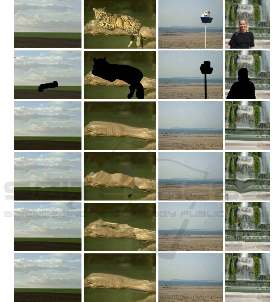
We now present some results on four different

images (ﬁgure 2). For each ﬁgure, the ﬁrst row

represents the original corrupted image, the sec-

ond one shows in black the mask to be inpainted.

Then we are presenting respectively the results from

(Tschumperl´e, 2006), the ones from (Bornemann and

M¨arz, 2007) and (Criminisi et al., 2004) and ﬁnally

the results of our algorithm.

By looking

at the results of the diffusion meth-

ods (row (c) and (d)), we observe the properties that

were already mentioned: these methods permit to ob-

tain regularized contours but are not able to recon-

struct the textures. Therefore the resulted images are

blurred. Remark that the method from (Tschumperl´e,

2006) gives better results than the one from (Borne-

mann and M¨arz, 2007) as it takes into account the

global geometry of the image and not only the most

important isophotes. When looking at the ﬁfth row,

we observe the opposite, textures are pretty well re-

constructed but the edges are not continuous. This

is particularly visible on the second of the fourth im-

ages, for which the gap is bigger.

For all the images, the results obtained with our

algorithm are very satisfactory. Indeed, our method

The properties of the results can be more easily noticed

by zooming on the images.

COMBINING TEXTURE SYNTHESIS AND DIFFUSION FOR IMAGE INPAINTING

(a)

(b)

(c)

(d)

(e)

(f)

Figure 2: Results of the proposed algorithm on four images. (a) Original image. (b) In black the mask to be inpainted. (c)

Results from (Tschumperl´e, 2006). (d) Results from (Bornemann and M¨arz, 2007). (e) Results from (Criminisi et al., 2004).

(f) Results from our algorithm.

combines the advantages of the two other types of ap-

proaches. Contrary to all the other techniques, there

is not any discontinuity on the boundary of the mask.

Furthermore, the textures are well propagated. Never-

theless, all these results are not perfect: the last image

still contains a bit of blur. Another drawback can be

highlighted from this result. Indeed, one can remark

that the result of the ﬁrst step of the algorithm, that is

the result of the diffusion method from (Tschumperl´e,

2006) inﬂuences the ﬁnal result. Therefore, if the re-

sult of this method is not satisfactory, the reconstruc-

tion given by our algorithm may contain more visual

artefacts.

VISAPP 2009 - International Conference on Computer Vision Theory and Applications

4 CONCLUSIONS

In this document, a state of the art of diffusion and

texture synthesis methods has ﬁrst been presented.

Some chosen algorithms have been described in more

detail and their results analysed. From this analy-

sis, it appeared judicious to combine a texture syn-

thesis method with a diffusion algorithm. Therefore,

we have proposed an algorithm that combines these

two types of approaches. It decomposes the origi-

nal image into the sum of a texture and a structure

image and inpaints each image independently. The

inpainted of the structure image is directly obtained

with the algorithm from (Tschumperl´e, 2006) while

for the completion of the texture image we have pro-

posed some extensions of the algorithm from (Crim-

inisi et al., 2004).

Some promising results have been shown. How-

ever, the quality of the results may still be improved,

as they depend on the diffusion method. Another

drawback is the inﬂuence of the parameters. The re-

sults presented were all obtained with the same pa-

rameters. Nevertheless, tuning them automatically

taking into account the type of data, would probably

improve the quality of our method. This will be the

topic of our future research.

ACKNOWLEDGEMENTS

This work was supported by the Torres Quevedo Pro-

gram of the Ministerio de Educaci´on y Ciencia of

Spain and partially founded by Mediapro through the

Spanish project CENIT-2007-1012 i3media.

REFERENCES

Ballester, C., Bertalm´ıo, M., Caselles, V., Sapiro, G., and

Verdera, J. (2001). Filling-in by joint interpolation

of vector ﬁelds and gray levels. IEEE Trans. on Im.

Processing, 10(8):1200–1211.

Bertalm´ıo, M. (2006). Strong-continuation, contrast-

invariant inpainting with a third-order optimal pde.

IEEE Trans. on Im. Processing, 15(7):1934–1938.

Bertalmio, M., Sapiro, G., Caselles, V., and Ballester, C.

(2000). Image inpainting. In SIGGRAPH: ACM Spe-

cial Interest Group on Comp. Graphics and Interac-

tive Techniques.

Bertalmio, M., Vese, L., Sapiro, G., and Osher, S. (2003).

Simultaneous structure and texture image inpainting.

IEEE Trans. on Im. Processing, 12(8):882–889.

Bornemann, F. and M¨arz, T. (2007). Fast image inpainting

based on coherence transport. Journal of Mathemati-

cal Imaging and Vis., 28(3):259–278.

Chan, T., Kang, S., and Shen, J. (2002). Euler’s elastica and

curvature based inpaintings. Journal of Appl. Math.,

63:564–592.

Chan, T., Osher, S., and Shen, J. (2001). The digital tv ﬁlter

and nonlinear denoising. IEEE Trans. on Im. Process-

ing, 10(2):231–241.

Chan, T. and Shen, J. (2001). Nontexture inpainting by

curvature-driven diffusions. Journal of Visual Com-

munication and Im. Representation, 12(4):436–449.

Criminisi, A., P´erez, P., and Toyama, K. (2004). Region ﬁll-

ing and object removal by exemplar-based inpainting.

IEEE Trans. on Im. Processing, 13(9):1200–1212.

Efros, A. and Leung, T. (1999). Texture synthesis by non-

parametric sampling. In In Proc. of the Int. Conf. on

Comp. Vis.

Harrison, P. (2001). A non-hierarchical procedure for re-

synthesis of complex textures. In WSCG Conf. Proc.

Masnou, S. (2002). Disocclusion: a variational approach

using level lines. IEEE Trans. on Im. Processing,

11(2):68–76.

Masnou, S. and Morel, J. (1998). Level-lines based dis-

occlusion. In Proceedings of 5th IEEE Intl Conf. on

Image Process., Chicago, volume 3, pages 259–263.

Meyer, Y. (2001). Oscillating patterns in image processing

and nonlinear evolution equations. American Mathe-

matical Society, Providence, RI.

Mumford, D. (1994). Algebraic Geometry and its Appli-

cations, chapter Elastica and Computer Vision, pages

491–506. Chandrajit Bajaj, New York, Springer-

Verlag.

Sun, J., Yuan, L., Jia, J., and Shum, H. (2005). Image com-

pletion with structure propagation. In SIGGRAPH:

ACM Special Interest Group on Comp. Graphics and

Interactive Techniques.

Telea, A. (2004). An image inpainting technique based on

the fast marching method. Journal of graphics tools,

9(1):23–34.

Tschumperl´e, D. (2006). Fast anisotropic smoothing

of multi-valued images using curvature-preserving

pde’s. Int. Journal of Comp. Vis., 68(1):65–82.

Tschumperle, D. and Deriche, R. (2005). Vector-valued im-

age regularization with pdes: a common framework

for different applications. IEEE Trans. on Pat. Analy-

sis and Machine Intelligence, 27(4):506–517.

Vese, L. and Osher, S. (2003). Modeling textures with total

variation minimization and oscillating patterns in im-

age processing. Journal scientiﬁc Computing, 19(1-

3):553–572.

Weickert, J. (1998). Anisotropic diffusion in image process-

ing. Teubner Verlag, Stuttgart.

COMBINING TEXTURE SYNTHESIS AND DIFFUSION FOR IMAGE INPAINTING