
MULTI-CLASS FROM BINARY
Divide to conquer
Anderson Rocha and Siome Goldenstein
Institute of Computing
University of Campinas (Unicamp), Campinas, Brazil
Keywords:
Multi-class classification, Error correcting output codes, ECOC, Affine Bayes, Bayesian approach.
Abstract:
Several researchers have proposed effective approaches for binary classification in the last years. We can
easily extend some of those techniques to multi-class. Notwithstanding, some other powerful classifiers (e.g.,
SVMs) are hard to extend to multi-class. In such cases, the usual approach is to reduce the multi-class problem
complexity into simpler binary classification problems (divide-and-conquer). In this paper, we address the
multi-class problem by introducing the concept of affine relations among binary classifiers (dichotomies), and
present a principled way to find groups of high correlated base learners. Finally, we devise a strategy to reduce
the number of required dichotomies in the overall multi-class process.
1 INTRODUCTION
Supervised learning is a Machine Learning strategy to
create a prediction function from training data. The
task of the supervised learner is to predict the value
of the function for any valid input object after having
seen a number of training examples (Bishop, 2006).
Many supervised learning techniques are conceived
for binary classification (Passerini et al., 2004). How-
ever, a lot of real-world recognition problems often
require that we map inputs to one out of hundreds or
thousands of possible categories.
Several researchers have proposed effective ap-
proaches for binary classification in the last years.
Successful examples of such approaches are margin
and linear classifiers, decision trees, and ensembles.
We can easily extend some of those techniques to
multi-class problems (e.g., decision trees). However,
we can not easily extend to multi-class some others
powerful and popular classifiers such as SVMs. In
such situations, the usual approach is to reduce the
multi-class problem complexity into multiple simpler
binary classification problems. Binary classifiers are
more robust to the curse of dimensionality than multi-
class approaches. Hence, it is worth dealing with a
larger number of binary problems.
A class binarization is a mapping of a multi-class
problem onto several two-class problems (divide-and-
conquer) and the subsequent combination of their out-
comes to derive the multi-class prediction (Pedrajas
and Boyer, 2006). We refer to the binary classifiers as
base learners or dichotomies.
There are many possible approaches to reduce
multi-class to binary classification problems. We can
classify such approaches into three broad groups (Pu-
jol et al., 2006): (1) One-vs-All (OVA), (2) One-
vs-One (OVO), and (3) Error Correcting Out-
put Codes (ECOC). Also, the multi-class decomposi-
tion into binary problems usually contains three main
parts: (1) the ECOC matrix creation; (2) the choice of
the base learner; and (3) the decoding strategy.
Our focus here is on the creation of the ECOC ma-
trix and on the decoding strategy. For the creation of
the ECOC matrix, it is important to choose a feasible
number of dichotomies to use. In general, the more
base learners we use, the more complex is the overall
procedure. For the decoding strategy, it is essential to
choose a deterministic strategy robust to ties and er-
rors in the dichotomies’ prediction.
In this paper, we introduce a brand new way to
combine binary classifiers to perform large multi-
class classification. We present a new Bayesian
treatment for the decoding strategy, the Affine-Bayes
Multi-class. We propose a decoding approach based
on the conditional probabilities of groups of high-
correlated binary classifiers. For that, we introduce
323
Rocha A. and Goldenstein S.
MULTI-CLASS FROM BINARY - Divide to conquer.
DOI: 10.5220/0001777803230330
In Proceedings of the Fourth International Conference on Computer Vision Theory and Applications (VISIGRAPP 2009), page
ISBN: 978-989-8111-69-2
Copyright
c
2009 by SCITEPRESS – Science and Technology Publications, Lda. All rights reserved

the concept of affine relations among binary clas-
sifiers and present a principled way to find groups
of high correlated dichotomies. Furthermore, we
present a strategy to reduce the number of required
dichotomies in the multi-class process.
Contemporary Vision and Pattern Recognition
problems such as face recognition, fingerprinting
identification, image categorization, DNA sequencing
among others often have an arbitrarily large number
of classes to cope with. Finding the right descriptor
is just a first step to solve a problem. Here, we show
how to use a small number of simple, fast, and weak
or strong base learners to get better results, no matter
the choice of the descriptor. This is a relevant issue
for large-scale classification problems.
We validate our approach using data sets from the
UCI repository, NIST, Corel Photo Gallery, and the
Amsterdam Library of Objects. We show that our ap-
proach provides better results than OVO, OVA, and
ECOC approaches based on other decoding strate-
gies. Furthermore, we also compare our approach to
Passerini et al. (Passerini et al., 2004), who proposed
a Bayesian treatment for decoding assuming indepen-
dence among all binary classifiers.
2 STATE-OF-THE-ART
Most of the existing literature addresses one or more
of the three main parts of a multi-class decomposi-
tion problem: (1) the ECOC matrix creation; (2) the
dichotomies choice; and (3) the decoding.
In the following, let T be the team (set) of used
dichotomies D in a multi-class problem, and N
T
be
the size of T . Recall that N
c
is the number of classes
1
.
There are three broad groups for reducing multi-
class to binary: One-vs-All, One-vs-One, and Error
Correcting Output Codes based methods (Pedrajas
and Boyer, 2006).
1. One-vs-All (OVA). Here, we use N
T
= N
c
=
O(N
c
) binary classifiers (dichotomies) (Clark and
Boswell, 1991; Anand et al., 1995). We train the
i
th
classifier using all patterns of class i as pos-
itive (+1) examples and the remaining class pat-
terns as negative (−1) examples. We classify an
input example x to the class with the highest re-
sponse.
2. One-vs-One (OVO). Here, we use
N
T
=
N
c
2
= O(N
2
c
) binary classifiers.
We train the ij
th
dichotomy using all patterns
of class i as positive and all patterns of class j
as negative examples. In this framework, there
1
In the Appendix, we provide a table of symbols.
are many approaches to combine the obtained
outcomes such as voting, and decision directed
acyclic graphs (DDAGs) (Platt et al., 1999).
3. Error Correcting Output Codes (ECOC). Pro-
posed by Dietterich and Bakiri (Dietterich and
Bakiri, 1996), in this approach, we use a coding
matrix M ∈ {−1, 1}
N
c
×N
T
to point out which
classes to train as positive and negative examples.
Allwein et al. (Allwein et al., 2000) have extended
such approach and proposed to use a coding ma-
trix M ∈ {−1, 0 , 1}
N
c
×N
T
. In this model, the
j
th
column of the matrix induces a partition of
the classes into two meta-classes. An instance x
belonging to a class i is a positive instance for
the j
th
dichotomy if and only if M
ij
= +1.
If M
ij
= 0, then it indicates that the i
th
class
is not part of the training of the j
th
dichotomy.
In this framework, there are many approaches
to combine the obtained outcomes such as vot-
ing, Hamming and Euclidean distances, and loss-
based functions (Windeatt and Ghaderi, 2003).
When the dichotomies are margin-based learners,
Allwein et al. (Allwein et al., 2000) have showed
the advantage and the theoretical bounds of us-
ing a loss-based function of the margin. Klau-
tau et al. (Klautau et al., 2004) have extended such
bounds to other functions.
Pedrajas et al. (Pedrajas and Boyer, 2006) have
proposed to combine the strategies of OVO and
OVA. Although the combination improves the over-
all multi-class effectiveness, the proposed approach
uses N
T
=
N
c
2
+ N
c
= O(N
2
c
) dichotomies
in the training stage. Moreira and Mayoraz (Mor-
eira and Mayoraz, 1998) also developed a combi-
nation of different classifiers. They have consid-
ered the output of each dichotomy as a probability
of the pattern of belonging to a given class. This
method requires
N
c
(N
c
+1)
2
= O(N
2
c
) base learners.
Athisos et al. (Athisos et al., 2007) have proposed
class embeddingsto choose the best dichotomies from
a set of trained base learners.
Pujol et al. (Pujol et al., 2006) have pre-
sented a heuristic method for learning ECOC ma-
trices based on a hierarchical partition of the class
space that maximizes a discriminative criterion.
The proposed technique finds the potentially best
N
c
− 1 = O(N
c
) dichotomies to the classifi-
cation. Crammer and Singer (Crammer and Singer,
2002) have proven that the problem of finding opti-
mal discrete codes is NP-complete. Hence, Pujol et al.
have used a heuristic solution for finding the best can-
didate dichotomies. Even such solution is computa-
tionally expensive, and the authors only report results
for N
c
≤ 28.
VISAPP 2009 - International Conference on Computer Vision Theory and Applications
324

Takenouchi and Ishii (Takenouchi and Ishii, 2007)
have used the information transmission theory to
combine ECOC dichotomies. The authors use the
full coding matrix M for the dichotomies, i.e.,
N
T
=
3
N
c
−2
N
c
+1
+1
2
= O(3
N
c
) dichotomies. The
authors only report results for N
c
≤ 7 classes.
Young et al. (Young et al., 2006) have used dy-
namic programming to design an one-class-at-a-time
removal sequence planning method for multi-class
decomposition. Although their approach only re-
quires N
T
= N
c
−1 dichotomies in the testing phase,
the removal policy in the training phase is expensive.
The removal sequence for a problem with N
c
classes
is formulated as a multi-stage decision-making prob-
lem and requires N
c
− 2 classification stages. In the
first stage, the method uses N
c
dichotomies. In each
one of the N
c
− 3 remaining stages, the method uses
N
c
(N
c
−1)
2
dichotomies. Therefore, the total number
of required base learners are
N
3
c
−4N
2
c
+5N
c
2
= O(N
3
c
).
Passerini et al. (Passerini et al., 2004) have intro-
duced a decoding function that combines the margins
through an estimate of their class conditional proba-
bilities. The authors have assumed that all base learn-
ers are independent and solved the problem using a
Na¨ıve Bayes approach. Their solution works regard-
less of the number of selected dichotomies and can be
associated with each one of the previous approaches.
3 AFFINE-BAYES MULTI-CLASS
In this section, we present our new Bayesian treat-
ment for the decoding strategy: the Affine-Bayes
Multi-class. We propose a decoding approach based
on the conditional probabilities of groups of affine bi-
nary classifiers. For that, we introduce the concept of
affine relations among binary classifiers, and present
a principled way to find groups of high correlated di-
chotomies. Finally, we present a strategy to reduce
the number of required dichotomies in the multi-class
classification.
To classify an input, we use a team of trained base
learners T . We call O
T
a realization of T . Each
element of T is a binary classifier (dichotomy) and
produces an output ∈ {−1, +1}. Given an input el-
ement x to classify, a realization O
T
contains the in-
formation to determine the class of x. In other words,
P (y = c
i
|x) = P (y = c
i
|O
T
).
However, we do not have the probability
P (y = c
i
| O
T
). From Bayes theorem,
P (y = c
i
|O
T
) =
P (O
T
|y = c
i
)P (y = c
i
)
P (O
T
)
∝ P (O
T
|y = c
i
)P (y = c
i
) (1)
P (O
T
) is just a normalizing factor and it is sup-
pressed.
Previous approaches have solved the above model
by considering the independence of the dichotomies
in the team T (Passerini et al., 2004). If we con-
sider independence among all dichotomies, the model
in Equation 1 becomes
P (y = c
i
|O
T
) ∝
Y
t ∈ T
P (O
t
T
|y = c
i
)P (y = c
i
),
(2)
and the class of the input x is
cl(x) = arg max
i
Q
t ∈ T
P (O
t
T
|y = c
i
)P (y = c
i
).
Although the independence assumption simplifies
the model, it comes with limitations and it is not the
best choice in all cases (Narasimhamrthy, 2005). In
general, it is quite difficult to solve independence
without using smoothing functions to deal with
numerical instabilities when the number of terms in
the series is too large. In such cases, it is necessary
to find a suitable density distribution to describe the
data, making the solution more complex.
We relax the assumption of independence among
all binary classifiers. When two of these dichotomies
have a lot in common, it would be unwise to threat
their results as independent random variables (RVs).
In our approach, we find groups of affine classifiers
(high correlated dichotomies) and represent their out-
comes as dependent RVs, using a single conditional
probability table (CPT) as an underlying distribution
model. Each group then has its own CPT, and we
combine the groups as if they are independent from
each other — to avoid a dimensionality explosion.
Our technique can be interpreted as a Bayesian
Network inspired approach for RV estimation. We
decide the RV that represent the class based on the
RVs that represent the outcomes of the dichotomies.
We model the multi-class classification problem
conditioned to groups of affine dichotomies G
D
. The
model in Equation 1 becomes
P (y = c
i
|O
T
, G
D
) ∝ P (O
T
, G
D
|y = c
i
)P (y = c
i
).
(3)
We assume independence only among the groups of
affine dichotomies g
i
∈ G
D
. Therefore, the class of
an input x is given by
cl(x) = arg max
j
Y
g
i
∈ G
D
P (O
g
i
T
, g
i
|y = c
j
)P (y = c
j
).
(4)
To find the groups of affine classifiers G
D
, we define
an affinity matrix A among the classifiers. The affin-
ity matrix measures how affine are two dichotomies
when classifying a set of training examples X. In
Section 3.1, we show how to create the affinity ma-
trix A. After calculating the affinity matrix A, we use
MULTI-CLASS FROM BINARY - Divide to conquer
325

a clustering algorithm to find the groups of correlated
binary classifiers in A. In Section 3.2, we show how
to find the groups of affine dichotomies from an affin-
ity matrix A.
The groups of affine classifiers can contain classi-
fiers that do not contribute significantly to the overall
classification. Therefore, we can deploy a procedure
to identify the less important dichotomies within an
affine group and eliminate them. In this stage, we are
able to reduce the number of required dichotomies
to perform the multi-class classification and hence
speed-up the overall process and make robust CPTs
estimations. In Section 3.3, we show a consistent
approach to eliminate the less important dichotomies
within an affine group.
In Algorithm 1, we present the main steps of our
model for multi-class classification. In line 1, we di-
vide the training data into five parts and use four parts
to train the dichotomies and one part to validate the
trained dichotomies and to construct the conditional
probability tables. In lines 3–6, we train and validate
each dichotomy using a selected method. The method
can be any binary classifier such as LDA, or SVM.
Each dichotomy produces an output ∈ {−1, +1 } for
each input x. In line 8, O contains all realizations of
the available dichotomies for the input data X
′
. In
lines 10 and 11, we find groups of affine dichotomies
using the realization O
i
. Using the information of
groups of affine dichotomies, in line 12, we create a
CPT for each affine group. These CPTs provide the
joint probabilities of a realization O
T
and the affine
groups g
i
⊂ G
D
when testing an unseen input data
x. In line 13, our approach finds the best dichotomies
within the affine groups. This information can be used
in the testing phase to reduce the number of used di-
chotomies.
3.1 Affinity Matrix A
Given a training data set X, we introduce a metric to
find the affinity between two dichotomies realizations
D
i
, D
j
whose outputs ∈ {−1, +1}
A
i,j
=
1
N
X
∀ x ∈ X
D
i
(x)D
j
(x)
, ∀ D
i
and D
j
∈ T .
(5)
According to the affinity model, if two dichotomies
have the same output for all elements in X, their affin-
ity is 1. For instance, this is the case when D
i
= D
j
.
If D
i
6= D
j
in all cases, their affinity is also 1. On
the other hand, if two dichotomies have half outputs
different and half equal, their affinity is 0. Using this
model, we can group binary classifiers that produce
similar outputs and, further, eliminate those which do
not contribute significantly to the overall classifica-
tion procedure.
Algorithm 1 Affine-Bayes Multi-class.
Require: Training data set X, Testing data X
t
, a team of
binary classifiers T .
1: Split X into k parts, X
i
such that i = 1 . . . k;
2: for each X
i
do ⊲ Inner k-fold cross-validation.
3: X
′
← X \ X
i
;
4: for each dichotomy d ∈ T do
5: D
train
← TRAIN(X
′
, d, method);
6: O
i
d
←TEST(X
i
, d, method, D
T rain
);
7: end for
8: O
i
←
S
(O
i
d
);
9: end for
10: Create the affinity matrix A for
S
O
i
;
11: Perform clustering on A to find the affine groups of
dichotomies G
D
;
12: Create a CPT for each group g ⊂ G
D
of affine di-
chotomies using O;
13: Perform the shrinking. GS
D
← SHRINK(G
D
);
14: for each x ∈ X
t
do
15: Perform the classification of x from the model
on Equation 4 either using the set of affine di-
chotomies G
D
or the shrinked GS
D
.
16: end for
3.2 Clustering
Given an affinity matrix A representing the relation-
ships among all dichotomies in a team T , we want to
find groups of classifiers that have similar affinities.
We want to find groups of dependent classifiers while
the groups are independent from one another. A good
clustering approach is important to provide balanced
groups of dichotomies. Such balancing is interesting
because it leads to simpler conditional probability ta-
bles. In this paper, we use a simple, yet effective,
greedy algorithm for finding the dependent groups of
dichotomies from the affinity matrix.
In our greedy clustering approach, first we find the
dichotomy with the highest affinity sum with respect
to all its neighbors (row with highest sum in A). Af-
ter that, we select the neighbors with affinity greater
or equal than a threshold t. Next, we check if each
dichotomy in the group is affine to the others and se-
lect those satisfying this requirement. This procedure
results the first affine group. Afterwards, we remove
the selected dichotomies from the main team T and
repeat the process until we analyze all available di-
chotomies. Throughout experiments, we have found
that t = 0.6 is a good threshold. We use this value in
all experiments in this paper.
VISAPP 2009 - International Conference on Computer Vision Theory and Applications
326

3.3 Shrinking
Sometimes, when modeling a problem using condi-
tional probabilities, we have to deal with large condi-
tional probability tables which can lead to over-fitting.
One approach to cope with this problem is to suppose
independence among all dichotomies which results
in the smallest possible CPT. However, as we show
in this paper, this approach limits the representative
power of the Bayes approach. In the following, we
show a clever and alternative approach.
In the shrinking stage, we want to find the di-
chotomies within a group that are more relevant for
the overall multi-class classification. We find the ac-
cumulative entropy of each classifier within a group
from the examples in the training data X. The higher
the accumulative entropy, the more representative is a
specific dichotomy. Let h
ij
be the accumulative en-
tropy for the classifier j within a group of affine di-
chotomies i. We define h
ij
as
h
ij
=
X
c∈C
L
X
x∈X
(p
cx
log
2
(p
cx
(1−p
cx
) log
2
(1− p
cx
)) (6)
where p
cx
= P (y = c | x, g
j
i
, O
g
j
i
x
), g
j
i
is the j
th
dichotomy within the affine group g
i
, O
g
j
i
x
is its real-
ization for the input x, and c ∈ C
L
the available class
labels.
We choose the classifiers with the highest cumu-
lative entropy to select the best classifiers within an
affine group. We have found in the experiments, that
selecting 60% of the classifiers is a good tradeoff be-
tween multi-class overall effectiveness and efficiency.
One could use another cutting criteria, such as the
maximum CPT size.
During the training phase, our approach finds the
affine groups of binary classifiers and marks the most
relevant dichotomies within each group. This infor-
mation can be used afterwards in the testing phase to
reduce the number of required classifiers in the multi-
class task.
In summary, with our solution, we measure the
affinity on the training data to learn the binary classi-
fiers relationship and decision surface. It is a simple
and fast way to estimate the distribution. Sometimes,
a dichotomy may be in the team because it is criti-
cal for discriminating between two particular classes.
If so, it is unlikely it will share a group of high-
correlated classifiers because it would require this di-
chotomy to be high-correlated with all dichotomies in
such group. We have performed some experiments
to test that and, in all tested cases, such dichotomies
specific for rare classes are kept in the final pool of
dichotomies.
4 EXPERIMENTS AND RESULTS
In this section, we compare our Affine-Bayes Multi-
class approach to: OVO, OVA, and ECOC approaches
based on distances decoding strategies. We also com-
pare our approach to Passerini et al. (Passerini et al.,
2004) who have proposed a Bayesian treatment for
decoding assuming independence among all binary
classifiers.
We validate our approach using two scenarios. In
the first scenario, we use data sets with a relative small
number of classes (N
c
< 30). For that, we use two
UCI
2
, and one NIST
3
data sets. In the second sce-
nario, we have considered two large-scale multi-class
applications: one for the Corel Photo Gallery (Corel)
4
data set and one for the Amsterdam Library of Ob-
jects (ALOI)
5
. Table 1 presents the main features of
each data set we have used in the validation. Recall
that, N
c
is the number of classes, N
d
if the number of
features, and N is the number of instances.
Table 1: Data sets’ summary.
Data set Source N
c
N
d
N
Mnist digits NIST 10 785 10,000
Vowel UCI 11 10 990
Isolet UCI 26 617 7,797
Corel Corel 200 128 20,000
ALOI ALOI 1,000 128 108,000
In the ECOC-based experiments, we have selected
15 random coding matrices. For each coding matrix,
we perform 5-fold cross validation. For each cross-
validation fold, we perform a 5-fold cross validation
on the training set to estimate the CPTs. In all exper-
iments, we have used the base learners: Linear Dis-
criminant Analysis (LDA) and Support Vector Ma-
chines (SVMs) (Bishop, 2006).
4.1 Scenario 1 (10–26 Classes)
In Figure 1, we compare Affine-Bayes (AB) to
ECOC based on Hamming decoding (ECOC),
One-vs-One (OVO), and Passerini’s approach
(PASSERINI) (Passerini et al., 2004). In this ex-
periment, Affine-Bayes uses two different coding
matrices: AB-ECOC, and AB-OVO.
The use of conditional probabilities and affine
groups on Affine-Bayes to decode the binary classifi-
cations and produce a multi-class prediction improves
the results for OVO and ECOC coding matrices. This
2
http://mlearn.ics.uci.edu/MLRepository.html
3
http://yann.lecun.com/exdb/mnist/
4
http://www.corel.com
5
http://www.science.uva.nl/˜aloi/
MULTI-CLASS FROM BINARY - Divide to conquer
327

Accuracy (%)
Number of Base Learners (N
T
)
AB-ECOC
ECOC
AB-OVO
OVO
PASSERINI
0
5 10 15
20
20
25 30
30
35 40
40
45
50
60
65
70
80
90
(a) Mnist .:. Base-learner = LDA.
Accuracy (%)
Number of Base Learners (N
T
)
AB-ECOC
ECOC
AB-OVO
OVO
PASSERINI
0
10
10
20
20
30
30
40
40
50
50
60
60
70
80
(b) Vowel .:. Base-learner = LDA.
Accuracy (%)
Number of Base Learners (N
T
)
AB-ECOC
ECOC
AB-OVO
OVO
PASSERINI
0
10
18
20
30
40
50
50
60
70
80
90
100
150
200 250 300
(c) Isolet .:. Base-learner = LDA.
Accuracy (%)
Number of Base Learners (N
T
)
AB-ECOC
ECOC
AB-OVO
OVO
PASSERINI
0
10
20
30
40
50
50
60
70
80
90
100
150
200 250 300
(d) Isolet .:. Base-learner = SVM.
Figure 1: Affine-Bayes (AB) vs. ECOC vs. OVO vs. Passerini for Mnist, Vowel, and Isolet data sets considering LDA and
SVM base learners.
is also true for other UCI data sets not shown here
such as abalone, covtype, optdigits, pendigits, vowel,
and yeast. Although unsubstantiated here, through-
out experiments we have found out that Affine-Bayes
also improves OVA and ECOC approaches limited to
N
T
= N
c
dichotomies.
Weak classifiers (e.g., LDA) benefits more from
Affine-Bayes than strong ones (e.g., SVMs). This im-
portant result shows us that when we have a problem
with many classes, it may be worth using weak clas-
sifiers (e.g., LDA) which often are considerably faster
than strong ones (e.g., SVMs).
When possible, all one-by-one dichotomies
(OVO) produce better results. However, random se-
lection of subsets of OVO are not better than ECOC,
and Affine-Bayes improves both approaches.
For the UCI and Nist small data sets, the Affine
Bayes results are, in average, one standard devia-
tion above Passerini’s results when using SVM and,
at least, two standard deviations above when using
LDA. However, we have found that Passerini’s as-
sumption on independence for all dichotomies is not
as robust as Affine-Bayes when the number of di-
chotomies and classes becomes larger (c.f., Sec. 4.2).
For small data sets, there is no much gain in using
anything sophisticated.
This behavior is closely related to the curse of di-
mensionality, and most papers in the literature only
show the performance going up to 30 classes which is
not useful for large-scale problems. Here, we validate
our approach for up to 1,000 classes.
4.2 Scenario 2 (200 and 1,000 Classes)
Here, we consider two large-scale Vision applica-
tions: Corel (N
c
= 200) and ALOI (N
c
= 1, 000)
categorization. In such applications, OVO is com-
putationally expensive. Sometimes, it is not advised
to use OVA at all, given that, even in this case,
the number of dichotomies and the number of el-
ements to train are too high. Hence, ECOC ap-
proaches with a few base learners are more appropri-
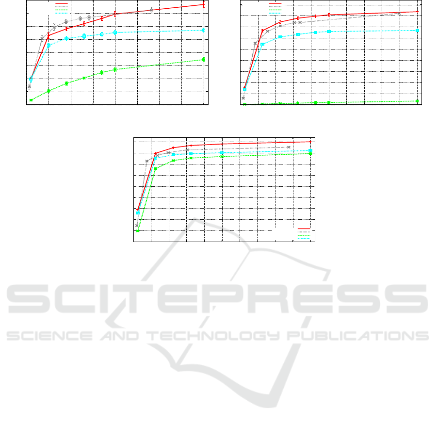
ate. In Figures 2(a–c), we show results using Affine-
Bayes (AB-ECOC) vs. ECOC Hamming decoding
and Passerini et al. (Passerini et al., 2004) approaches
for LDA and SVM classifiers.
We show experiments up to 400 dichotomies in
the presence of 200 and 1,000 classes to emphasize
the performance for a small number of base learners
in comparison with the number of all possible separa-
tion choices. As we increase the number of classifiers,
all approaches fare steadily better, and as this number
approaches the limit, they converge to similar results.
For ALOI, the limit is
1,000
2
= 499, 500, much more
than the 400 we show.
As the image descriptor is not our focus in this pa-
VISAPP 2009 - International Conference on Computer Vision Theory and Applications
328
Accuracy (%)
Number of Base Learners (N
T
)
AB-ECOC
ABS-ECOC
ECOC
PASSERINI
0
0
3
6
9
12
15
18
21
24
50
100 150 200
250
300 350 400
(a) Corel Gallery .:. Base-learner = LDA.
Accuracy (%)
Number of Base Learners (N
T
)
AB-ECOC
ABS-ECOC
ECOC
PASSERINI
0
0
10
20
30
40
40
50
60
70
80
80
90
120
160
200 240
280
320 360 400
(b) ALOI .:. Base-learner = LDA.
Accuracy (%)
Number of Base Learners (N
T
)
AB-ECOC
ABS-ECOC
ECOC
PASSERINI
0
0
10
20
30
40
40
50
60
70
80
80
90
120 160 200 240 280
320
360 400
(c) ALOI .:. Base-learner = SVM.
Figure 2: Affine-Bayes (AB) and Affine-Bayes-Shrinking (ABS) vs. ECOC vs. Passerini for two large-scale data sets.
per, we have used a simple extended color histogram
with 128 dimensions (Stehling et al., 2002). Corel
data set comprises broad-class images and it is more
difficult to classify than the ALOI collection of con-
trolled objects.
Affine-Bayes improves the effectiveness in the two
data sets regardless the base learner (LDA or SVM).
In both cases and for both data sets, we see that
Affine-Bayes provides better results than Passerini’s
and other approaches. For ALOI and SVM base
learner, the difference is above 15 standard deviations
(∼7–8 percentual points) with respect to Passerini’s
results.
In addition, Affine-Bayes with the shrinking phase
provides good results even with fewer dichotomies.
For instance, when we provide 200 dichotomies in
the training for ALOI data set, Affine-Bayes (AB) pro-
vides an average accuracy of 80% while Affine-Bayes-
Shrinking (ABS) provides 76% using only 135 di-
chotomies. For Corel, when we use AB with 90 di-
chotomies, the accuracy is 17% while for ABS it is
18%. Finally, in spite of the reduction in the num-
ber of dichotomies, Affine-Bayes still provides better
effectiveness than previous approaches.
For more than 30 classes, the independence re-
striction play an important role. See Figure 2(b-c).
By not assuming independence, the SVM with only
200 dichotomies is more effective than the best K-
Nearest neighbors (not shown in the plots). KNN
yields ≈ 83% accuracy while our approach using
SVM and 200 dichotomies yields ≈ 88%. We can
improve even more if we use 400 dichotomies, and
yet, this is much less dichotomies than a solution us-
ing one versus all or all combinations of one versus
one.
5 CONCLUSIONS AND
REMARKS
In this paper, we have addressed two key issues of
multi-class classification: the choice of the coding
matrix and the decoding strategy. For that, we have
presented a new Bayesian treatment for the decoding
strategy: Affine-Bayes.
We have introduced the concept of affine relations
among binary classifiers and presented a principled
way to find groups of high correlated base learners.
Furthermore, we have presented a strategy to reduce
the number of required dichotomies in the multi-class
process.
The advantages of our approach are: (1) it works
independent of the number of selected dichotomies;
(2) it can be associated with each one of the previ-
MULTI-CLASS FROM BINARY - Divide to conquer
329

ous approaches such as OVO, OVA, ECOC, and their
combinations; (3) it does not rely on the independence
restriction among all dichotomies. (4) its implemen-
tation is simply and it uses only basic probability the-
ory; (5) it is fast and does not impact the multi-class
procedure.
Future work include the deployment of better poli-
cies to choose the coding matrix and the design of
alternative ways to store the conditional probability
tables other than sparse matrices and hashes.
ACKNOWLEDGEMENTS
We thank FAPESP (Grant 05/58103-3), and CNPq
(Grants 309254/2007-8 and 551007/2007-9) for the
financial support.
REFERENCES
Allwein, E., Shapire, R., and Singer, Y. (2000). Reducing
multi-class to binary: A unifying approach for margin
classifiers. JMLR, 1(1):113–141.
Anand, R., Mehrotra, K., Mohan, C., and Ranka, S. (1995).
Efficient classification for multi-class problems using
modular neural networks. TNN, 6(1):117–124.
Athisos, V., Stefan, A., Yuan, Q., and Sclaroff, S. (2007).
Classmap: Efficient multiclass recognition via embed-
dings. In ICCV.
Bishop, C. (2006). Pattern Recognition and Machine
Learning. Springer, 1 edition.
Clark, P. and Boswell, R. (1991). Rule induction with CN2:
Some improvements. In EWSL, pages 151–163.
Crammer, K. and Singer, Y. (2002). On the learnability
and design of output codes for multi-class problems.
JMLR, 47(2–3):201–233.
Dietterich, T. and Bakiri, G. (1996). Solving multi-class
problems via ECOC. JAIR, 2(1):263–286.
Klautau, A., Jevtic, N., and Orlitsky, A. (2004). On nearest-
neighbor ECOC with application to all-pairs multi-
class support vector machines. JMLR, 4(1):1–15.
Moreira, M. and Mayoraz, E. (1998). Improved pairwise
coupling classification with correcting classifiers. In
ECML.
Narasimhamrthy, A. (2005). Theoretical bounds of majority
voting performance for a binary classification prob-
lem. TPAMI, 27(12):1988–1995.
Passerini, A., Pontil, M., and Frasconi, P. (2004). New re-
sults on error correcting output codes of kernel ma-
chines. TNN, 15(1):45–54.
Pedrajas, N. and Boyer, D. (2006). Improving multi-class
pattern recognition by the combination of two strate-
gies. TPAMI, 28(6):1001–1006.
Platt, J., Christiani, N., and Taylor, J. (1999). Large mar-
gin dags for multi-class classification. In NIPS, pages
547–553.
Pujol, O., Radeva, P., and Vitria, J. (2006). Discriminant
ECOC: A heuristic method for application dependent
design of ECOC. TPAMI, 28(6):1007–1012.
Stehling, R., Nascimento, M., and Falc˜ao, A. (2002). A
compact and efficient image retrieval approach based
on border/interior pixel classification. In CIKM, pages
102–109.
Takenouchi, T. and Ishii, S. (2007). Multi-class classifica-
tion as a decoding problem. In FOCI, pages 470–475.
Windeatt, T. and Ghaderi, R. (2003). Coding and decoding
strategies for multi-class learning problems. Informa-
tion Fusion, 4(1):11–21.
Young, C., Yen, C., Pao, Y., and Nagurka, M. (2006). One-
class-at-time removal sequence planning method for
multi-class problems. TNN, 17(6):1544–1549.
APPENDIX
Table 2: List of useful symbols.
X, x Data samples, and an element of X.
Y , y The class’ labels of X and an element of Y .
N Number of elements of X.
N
c
Number of classes.
N
d
The dimensionality X.
C
L
, c The class labels and a class such that c
i
∈ C
L
.
Ω All possible dichotomies for C.
T A team of dichotomies such that T ⊂ Ω.
N
T
The number of dichotomies in T .
M A coding matrix
O
T
A realization of T .
A The affine matrix.
G
D
The groups of affine dichotomies.
g
i
Group of affine dichotomies such that g
i
⊂ G
D
.
VISAPP 2009 - International Conference on Computer Vision Theory and Applications
330
