
REAL-TIME MULTI-OBJECT TRACKING WITH FEW PARTICLES
A Parallel Extension of MCMC Algorithm
Franc¸ois Bardet, Thierry Chateau and Datta Ramadasan
LASMEA, Universit
´
e Blaise Pascal, 24 avenue des Landais, F-63177 Aubi
`
ere cedex, France
Keywords:
Multi-object tracking, MCMC particle filter, Parallel computing, Real time.
Abstract:
This paper addresses real-time automatic tracking and labeling of a variable number of generic objects, using
one or more static cameras. The multi-object configuration is tracked through a Markov Chain Monte-Carlo
Particle Filter (MCMC PF) method. As this method sequentially processes particles, it cannot be speeded up
by parallel computing allowed by multi-core processing units. As a main contribution, we propose in this
paper an extended MCMC PF algorithm, benefiting from parallel computing, and we show that this strategy
improves tracking operation. This paper also addresses object tracking involving occlusions, deep scale and
appearance changes: we propose a global observation function allowing to fairly track far objects as well as
close objects. Experiment results are shown and discussed on pedestrian and on vehicle tracking sequences.
1 INTRODUCTION
Real-time visual tracking of a variable number of ob-
jects is of high interest for several applications such as
visual surveillance of people, animals or vehicles. In
the recent years, several works addressed these fields,
showing interesting results. Among others: tracking
up to 4 pedestrians involving occlusions (Isard and
MacCormick, 2001), multiple vehicle tracking from a
low elevation camera (yielding occlusions) (Kanhere
and Birchfield, 2005), tracking up to 20 ants from a
top view (Khan et al., 2005). The work presented
below is closely inspired by the latter, extended to
a generic tracker where deep occlusions frequently
occur, and where object and background appearance
may change. We also want the tracker to operate upon
any kind of opaque generic objects (modeled by a
cuboid), requiring no ad-hoc features but only object
dimensions and its dynamics model if any (in case of
a vehicle). Designing a multi-object tracker comply-
ing with these requirements is still challenging.
Particle Filters belong to the class of Monte-Carlo
recursive Bayesian filters, and is of popular use in
the field of object tracking, because Particle Filters
can cope with non-linearities and multi-modalities in-
duced by occlusions and background clutter. As a
sampled method, Particle Filters require a way to
smartly choose and propagate the samples (the ”par-
ticles”) over time. As the system state may evolve
at each time step, samples must be moved adap-
tatively towards the most informing regions of the
state space. This is a sequential adaptive resam-
pling method known as SIR algorithm (Sample Im-
portance Resampling) (M. Isard and A. Blake, 1998).
A monocular multi-object tracker based on it was pro-
posed (Isard and MacCormick, 2001), and many other
works followed. The drawback of SIR, shown by
many authors (Isard and MacCormick, 2001; Smith,
2007), is that it can’t deal with high-dimensional
state-spaces, because the number of required particles
grows as an exponential of the state-space dimension.
Thus, a SIR Particle Filter can’t track more than 2 or
3 objects. Partitionned Particle Filter (MacCormick
and Blake, 1999) has been proposed to overcome this
limitation, but it processes objects by order, yielding
to unfairly tracking them (Smith, 2007). An off-line
non-sequential approach, when real-time is not re-
quired, uses a Markov Chain Monte-Carlo state space
exploration to associate data in order to track objects
over a whole sequence (Yu et al., 2007). For real-time
tracking, Markov Chain Monte-Carlo Particle Filters
(MCMC PF) have been shown to successfully track
2 to 4 pedestrians (Smith, 2007). More objects (up
to 20 ants) (Khan et al., 2005) have successfully been
tracked in a case where occlusions are avoided (top
view of ants walking on a planar ground). Both em-
phasized the benefit of MCMC PF: the required num-
ber of particles is only a linear function of the number
of tracked objects, when they do not interact. More
computation is only required in case objects interact
456
Bardet F., Chateau T. and Ramadasan D.
REAL-TIME MULTI-OBJECT TRACKING WITH FEW PARTICLES - A Parallel Extension of MCMC Algorithm.
DOI: 10.5220/0001779104570464
In Proceedings of the Fourth International Conference on Computer Vision Theory and Applications (VISIGRAPP 2009), page
ISBN: 978-989-8111-69-2
Copyright
c
2009 by SCITEPRESS – Science and Technology Publications, Lda. All rights reserved

(i.e. occlude). In this case, real time tracking of sev-
eral objects yet is a challenge. As a main contribution,
we propose in this paper an extended MCMC PF al-
gorithm, benefiting from parallel computing, and we
show that this strategy improves tracking operation.
To address object occlusions and deep scale changes,
we also propose in this paper a global observation
function allowing to fairly track far objects as well
as close objects. Experiment results are shown and
discussed on pedestrian and on vehicle tracking se-
quences. This paper is organised as follows: in sec-
tion 2, we develop the MCMC PF method for track-
ing a variable number of objects. In section 3, we
extend the MCMC PF method in order to benefit of
multi-core processing units. In section 4, we describe
the observation function, focusing on their indepen-
dance to scale change. In section 5, tracking results
are demonstrated and discussed with a focus on real-
time capabilities.
2 MULTI-OBJECT MCMC PF
Let p(X
t
|Z
1:t
) denote the posterior probability den-
sity for a system state to be X
t
at time t, knowing
an observation sequence Z
1:t
. Particle Filters prop-
agate a number N of particles over time, to approx-
imate p(X
t
|Z
1:t
) as a sum of Dirac functions, such
that: p(X
t
|Z
1:t
) ≈
1
N
∑
N
n=1
δ(X
t
− X
n
t
) where X
n
t
de-
notes the n-th state sample at time t. In MCMC
Particle Filters, these samples are drawn iteratively,
through a first order Markov process.
2.1 State Space
In object tracking the state encodes the configura-
tion of the perceptible objects: X
n
t
= {I
n
t
,x
n
t,i
}, i ∈
{1,..., I
n
t
}, where I
n
t
is the number of visible objects
for hypothesis n at time t, n ∈ {1, ...,N} where N is
the number of iterations, and x
n
t,i
is a vector encoding
the state of object i, such that x
n
t,i
= {p
n
t,i
,v
n
t,i
,s
n
t,i
,a
n
t,i
}.
The object i position at iteration n is described by p
n
t,i
,
a 3-component vector including the 2D ground pro-
jection of the object center of gravity, and its orienta-
tion angle. The ground is assumed to be planar. The
object velocity is described by v
n
t,i
, a 2-component
vector including the velocity magnitude and orien-
tation. Its shape is described by s
n
t,i
, a 3-component
vector including width, length and height of a cuboid
approximating the object shape. a
n
t,i
denotes its ap-
pearance vector, helping to maintain object identity.
We use the color model proposed in (P. Perez et al.,
2002): we convert our images to a hue-saturation-
value color space, then pixels with sufficient value
(b): P-proposal MCMC(a): single proposal MCMC
X
n
X
n−1
π
n−1
π
n
π
∗
X
∗
α
1 − α
X
n
X
n−1
π
n−1
π
n
α
1 − α
X
∗
1
π
∗
1
π
∗
P
X
∗
P
X
∗
p
π
∗
p
p ∈ {1, ..., P }
Figure 1: (a): one step of algorithm 1 produces a unique
proposal X
∗
, accepted as next state X
n
with probability α. If
rejected then X
n
= X
n−1
. (b): one step of algorithm 2 pro-
duces P proposals X
∗
p
. One of them is drawn by importance
sampling according to weights π
∗
p
, then accepted as next
state X
n
with probability α. If rejected then X
n
= X
n−1
.
and saturation feed an unmarginalized hue-saturation
histogram, other pixels a value histogram. Both are
concatenated to build a color model whose benefit is
a lesser sensitivity to illumination changes.
2.2 MCMC PF for Multi-Object
Tracking
MCMC PF for tracking a variable number of objects
was introduced in (Khan et al., 2005), and is described
in algorithm 1. Omitting time t for sake of simplicity,
figure 1-a focuses on the markovian transition from
particle X
n−1
to particle X
n
via a unique new proposal
X
∗
, which may be accepted with probability α (de-
fined in algorithm 1). If refused then X
n
is a duplicate
of X
n−1
. This is the Metropolis-Hastings acceptance
rule (MacKay, 2003). Please note that computing pro-
posal X
∗
likelihood π
∗
is by far the heaviest step in the
algorithm, as it involves image wide computations.
2.3 Marginalized Proposal Moves
Basic Particle Filters (i.e. those which draw new sam-
ples by moving jointly along all the dimensions) can’t
cope with a high dimension state space, because the
required number of samples grows as an exponential
of the space dimension, as focused in (Smith, 2007).
The best issue to this problem would be to process
Metropolis-Hastings algorithm with a proposal move
on only one randomly chosen dimension at each itera-
tion. We cannot choose this optimal solution, because
the components of p
n
t,i
and s
n
t,i
are not independantly
observable. For that reason, we chose a midway solu-
tion: the transition from state hypothesis X to the next
X
∗
, is conditionned by a proposal density q(X
∗
|X), al-
lowing changes along all the dimensions of one ran-
domly chosen object at a time, within its own state
subspace. This solution was also chosen by other au-
thors (Khan et al., 2005; Smith, 2007).
REAL-TIME MULTI-OBJECT TRACKING WITH FEW PARTICLES - A Parallel Extension of MCMC Algorithm
457

Table 1: Prior object dimensions.
pedestrian mini maxi
length (m) 0.15 0.3
width (m) 0.25 0.45
height (m) 1.2 2.0
velocity magnitude (m.s
−1
) 1 2
velocity angle (deg) 0 360
vehicle mini maxi
length (m) 3.5 5.5
width (m) 1.4 2
height (m) 1.4 2.2
velocity magnitude (m.s
−1
) 10 30
velocity angle (deg) -30 +30
2.4 Variable Number of Objects
To allow the number of objects to change, authors in-
troduced RJMCMC (Reversible Jump Markov Chain
Monte Carlo) (Green, 1995). As the number of vis-
ible objects may change, the state space dimension
also may change, the state may thus ”jump” from a
subspace to another one of larger or smaller dimen-
sion if a new object enters or leaves the scene. To
prevent the search chain from getting stuck in a local
minimum, the jumps between subspaces must be re-
versible. For that reason, authors proposed the pair of
discrete reversible moves {enter,leave} (Khan et al.,
2005; Smith, 2007). To improve time consistency, ob-
ject leave proposals are driven by its life expectancy,
a continuous variable updated at each iteration as a
function of how the particle object matches the obser-
vation. The ob ject update move is self-reversible as
it is a continuous move. The whole move set will be
denoted as M = {enter,leave,ob ject update}.
2.5 Proposal Moves
Enter: Propose a new joint configuration X
∗
=
{X
n−1
,x
I
n−1
+1
}, adding a new object x
I
n−1
+1
to the
previous joint configuration X
n−1
, where I
n−1
is the
number of objects hypothesized by X
n−1
. Entering
object is given an initial life expectancy, and its priors
are given in table 1. The search process jumps to a
higher dimension state subspace.
Leave: The reverse move proposes to withdraw ob-
ject i from X
n−1
: propose X
∗
= {X
n−1
\ x
n−1
i
}, i ∈
{1,..., I
n−1
}, I
n−1
is hypothesis X
n−1
object number,
and {s \e} is set s without element e. The search pro-
cess jumps to a lower dimension state subspace.
Object Update: At each iteration n of time t Markov
chain, we randomly choose an object j to be updated
among particle X
n
t
. We randomly choose a time t − 1
particle X
r
t−1
, r ∈ {1,...,N}, also involving object j,
within the input set:{X
n
t−1
}
N
n=1
. From this object j
instance x
j,n
t−1
, we draw a position, velocity and shape
proposal, according to equations 1, 2, 3:
q(p
∗
|p
r
t−1
) = N (p
r
t−1
,σ
2
p
I
2
) (1)
q(v
∗
|v
r
t−1
) = N (v
r
t−1
,diag
σ
2
m
,σ
2
a
) (2)
q(s
∗
|s
r
t−1
) = N (s
r
t−1
,σ
2
s
I
3
) (3)
where σ
p
is the position standard deviation, σ
m
and
σ
a
are the respective velocity magnitude and orienta-
tion standard deviations, σ
s
is the shape standard de-
viation, I
d
is the d-dimension identity matrix.
Algorithm 1 MCMC Particle Filter.
Input: particle set at time t − 1: {X
n
t−1
}
N
n=1
Initialize the chain: X
0
t
= X
r
t−1
r ∈ {1,...,N}.
- Compute its likelihood: π
0
t
∝ P(Z
t
|X
0
t
).
for i = 1 to N + N
B
do
- Randomly draw a move m from move set M.
if m == ob ject update then
- Randomly choose object j in particle X
i−1
t
.
- Randomly choose X
n
t−1
, a particle involving
object j: x
j,n
t−1
from the input set:{X
n
t−1
}
N
n=1
.
- Apply dynamics to object x
j,n
t−1
: draw a sam-
ple x
j∗
t
from the evolution density q(x
∗
|x
j,n
t−1
).
- Build X
∗
replacing x
j,i−1
t
by x
j∗
t
as object j.
else
- Propose an enter: X
∗
= {X
i−1
t
,x
I
i−1
+1
}
end if
- Compute its likelihood: π
∗
∝ P(Z
t
|X
∗
).
- Compute the acceptance ratio :
α = min
1,
π
∗
q(X
i−1
t
|X
∗
)
π
i−1
t
q(X
∗
|X
i−1
t
)
- Add X
i
t
= X
∗
to the chain with probability α,
or X
i
t
= X
i−1
t
with probability 1 − α.
- Update object j life expectancy.
end for
Discard the N
B
first samples of the chain (burn-in).
Output: particle set at time t: {X
n
t
}
n=N
B
+1,...,N
B
+N
3 PARALLEL COMPUTING
WITHIN MCMC FRAMEWORK
Multi-processor systems and multi-core processing
units are now widely used. A multi-core unit can si-
multaneously process multiple independant tasks, so
VISAPP 2009 - International Conference on Computer Vision Theory and Applications
458
20 40 60
0
0.02
0.04
0.06
0.08
0.1
0.12
20 40 60
0
0.02
0.04
0.06
0.08
0.1
0.12
20 40 60
0
0.02
0.04
0.06
0.08
0.1
0.12
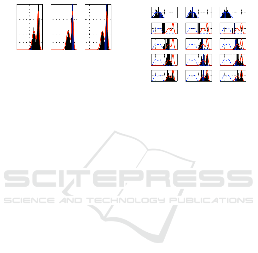
Figure 2: Sampling a monodimensional density function
(red solid line) on [0, 100] range, with a MCMC sampler
(histogram of particles in blue). Left: single proposal, cen-
ter: dual proposal, right: 4-proposal. N = 1000 iterations,
with iteration n proposal density: N (x
n−1
,5
2
).
the global power benefit is conditionned to the pos-
sibility to balance computation loads between cores.
In algorithm 1, the proposal likelihood computation
required is by far the heaviest step in terms of compu-
tation costs, as it involves image wide computations
(they will be detailed in section 4). Thus it is the best
candidate task to be parallelized. Unfortunately, this
task is required at every iteration of the chain, and its
result is used to decide whether the proposal should
be accepted or not as a new sample. Thus algorithm 1
cannot be parallelized as is.
In order to get benefit from parallel processors,
we propose an extended version of algorithm 1, si-
multaneously generating mutiple state proposals and
assessing their likelihoods. Algorithm 2 summerizes
the operations. We denote it MCMC
P
PF, where the
superscript
P
is the number of processing cores on
the machine processing unit. It differs from algo-
rithm 1 in the P time replication of the proposal and
evaluation mechanism, and in the additional impor-
tance sampling step that comes subsequently. Omit-
ting time t for sake of simplicity, figure 1-b illus-
trates one step of algorithm 2, a markovian transition
from particle X
n−1
to particle X
n
via P new propos-
als X
∗
p
, p ∈ {1,...,P}. Each processing core receives
one of these state proposals, evaluates its likelihood
π
∗
p
∝ P(Z
t
|X
∗
p
) and returns it to the main process. One
of them is then drawn by importance sampling among
all the parallel proposals and their associated likeli-
hoods π
∗
p
. It is accepted as next state X
n
with proba-
bility α. If rejected then X
n
is the duplicate of X
n−1
.
Figure 2 shows that single and multi-proposal
MCMC samplers similarly estimate any target den-
sity. Figure 3 shows that our MCMC
P
PF behaves
similarly regardless to the value of P. As a filter, it
smoothly starts moving from t = 1 towards the new
probability density. It also shows that multiple pro-
posal filters converge faster, allowing to reduce the
chain length.
20 40 60
0
0.05
0.1
MCMC
1
PF
t = 0
20 40 60
0
0.05
0.1
MCMC
2
PF
20 40 60
0
0.05
0.1
MCMC
4
PF
20 40 60
0
0.05
0.1
t = 1
20 40 60
0
0.05
0.1
20 40 60
0
0.05
0.1
20 40 60
0
0.05
0.1
t = 2
20 40 60
0
0.05
0.1
20 40 60
0
0.05
0.1
20 40 60
0
0.05
0.1
t = 3
20 40 60
0
0.05
0.1
20 40 60
0
0.05
0.1
20 40 60
0
0.05
0.1
t = 4
20 40 60
0
0.05
0.1
20 40 60
0
0.05
0.1
Figure 3: Filtering a monodimensional time-evolving den-
sity function (red solid line) on [0, 100] range, with a
MCMC
P
PFfilter (histogram of particles in blue). Left: sin-
gle proposal P = 1, center column: dual proposal P = 2,
right: 4-proposal P = 4. Steady state until t=0 (upper row).
At time t=1 (second row), density dramatically changes then
remains steady until t=4 (bottom row). N = 100 particles
with particle n proposal density: N (x
n−1
t−1
,5
2
).
4 OBSERVATION FUNCTION
4.1 Background Model
Though only one camera is used in many surveil-
lance applications, more cameras may be required,
either to increase the trajectory estimate accuracy, or
to increase the measurement range. For that reason,
our measurement function can merge data from one
or more cameras. Assuming still cameras and back-
ground, we first process a simple background subtrac-
tion on each frame. Then each pixel is classified as
background or foreground, and we compute a binary
foreground image according to equation 4:
I
F
(g,c) =
1 if p(z
g,c
|l
g,c
= F) > p(z
g,c
|l
g,c
= B)
0 otherwise
(4)
where z
g,c
denotes the pixel value at location g of
the frame sent by camera number c at time t, ∀g ∈
{1,..., G} with G the number of processed pixels of
the frame, ∀c ∈ {1, ...,C}, with C the number of cam-
eras in use, and l
g,c
∈ {B,F} is a label assigned to the
pixel at location g, according to whether the state hy-
pothesis X assumes that this pixel is illuminated either
by the Background B, or by a Foreground object F.
4.2 Global Observation Likelihood
Each object hypothesized by state X is modeled as a
cuboid with shape defined by s
n
t,i
as defined in section
REAL-TIME MULTI-OBJECT TRACKING WITH FEW PARTICLES - A Parallel Extension of MCMC Algorithm
459

Algorithm 2 MCMC
P
Particle Filter.
Input: particle set at time t − 1: {X
n
t−1
}
N
n=1
Initialize the chain: X
0
t
= X
r
t−1
r ∈ {1, ...,N}, and
its weight: π
0
t
) ∝ P(Z
t
|X
0
t
)
for i = 1 to N + N
B
do
for p = 1 to P do
- Randomly draw a move m from move set M
if m == ob ject update then
- Randomly choose object j
p
from X
i−1
t
.
- Randomly choose a particle involving ob-
ject j
p
: x
j
p
,n
t−1
from the input set:{X
n
t−1
}
N
n=1
.
- Apply dynamics to object x
j
p
,n
t−1
: draw x
j
p
∗
t
from the evolution density q(x
∗
|x
j
p
,n
t−1
).
- Build X
∗
p
replacing x
j
p
,i−1
t
by x
j
p
∗
t
.
else
- Propose an enter: X
∗
p
= {X
i−1
t
,x
I
i−1
+1
}
end if
- Compute its likelihood: π
∗
p
∝ P(Z
t
|X
∗
p
)
end for
-Sample one of the P proposals by importance
sampling among the weighted proposal set :
{X
∗
,π
∗
} ∝ {X
∗
p
,π
∗
p
}
P
p=1
- Compute the acceptance ratio :
α = min
1,
π
∗
q(X
i−1
t
|X
∗
)
π
i−1
t
q(X
∗
|X
i−1
t
)
- Add X
i
t
= X
∗
to the chain with probability α,
or X
i
t
= X
i−1
t
with probability 1 − α.
- Update object j life expectancy.
end for
Burn-in : discard the N
B
first samples of the chain.
Output: particle set at time t: {X
n
t
}
n=N
B
+1,...,N
B
+N
2.1. We compute the convex hull of its vertice projec-
tions into the camera images. We then compute for
each camera c a binary hypothesis image I
H
(X,g,c),
setting pixel g value to 1 if it is inside at least one of
the said convex hulls, else 0. A similarity image is
finally computed I
S
(X,g,c):
I
S
(X,g,c) =
1 if I
F
(g,c) = I
H
(X,g,c)
0 otherwise
(5)
∀g ∈ {1,...,G}, ∀c ∈ {1,...,C}.
Tracking multiple vehicles or pedestrians in traffic
involves deep scale changes due to projection. Thus
a naive image similarity ratio (the number of 1’s in
I
S
divided by its area) would be much more discrim-
inant for close object moves, than for further object
moves. This drawback is illustrated by figure 4, where
each object is proposed a horizontal move of half its
width. Almost every move of the smallest objects
would be accepted without discrimination. To solve
this problem, we propose an original object-area de-
pendent global observation likelihood, ensuring a tar-
get acceptance ratio, independantly to the object area.
This is made possible because algorithm 1 only moves
one hypothesized object at a time. We compute a pa-
rameter denoted β
c
∀c ∈ {1,...,C}, such that a given
relative loss of object coverage k
S
leads to a target
acceptance criterium α
t
. Let us denote S the area of
the foreground binary image I
F
, S
o,c
the moved ob-
ject area in camera c image. In our experiment, we
choose k
S
= 0.1 and α
t
= 0.5, meaning that an ob-
ject proposal covering only 90% of the previous hy-
pothesized object, would lead to an acceptance ratio
α
t
= 0.5, thus equiprobably accepting or refusing this
proposal. We compute the global likelihood as:
π
F,c
(X) =
1
S
∑
g∈{1,...,G}
I
S
(g,c)
β
c
∀c ∈ {1,...,C}
(6)
where π
F,c
(X) = 1 if the hypothesis mask I
H
(X) per-
fectly fits I
F
, and π
F,c
(X) =
S−2S
o,c
S
β
c
if they do not
intersect at all. The parameter β
c
can be computed as:
β
c
=
log(α
t
)
log(1 − 2k
S
S
o,c
S
)
(7)
Acceptance ratio no more depends on the object dis-
tance, as illustrated on figure 4. Remaining dispari-
ties are due to the object shapes which do not fit all
the same the hypothesized rectangles. This observa-
tion function gives us the opportunity to adjust the
Metropolis-Hastings acceptance rate, as it determines
the search efficiency. Finally the global configuration
X likelihood required to compute algorithms 1 or 2
acceptance rate, is calculated as:
π(X) =
C
∏
c=1
π
F,c
(X) (8)
5 EXPERIMENTS AND RESULTS
5.1 Synthetic Data Experiments
Particle filters are suitable to estimate any kind of
state and observation probability densities, without
any gaussian hypothesis, as illustrated on figure 2.
Nevertheless, in order to assess and compare algo-
rithms 1 and 2 efficiencies, we choose to use multi-
variate gaussian probability densities in order to al-
low the use of a Kalman Filter as a reference, as it is
known to be an optimal filter in such conditions. This
test is based on fully synthetic data, as defined below:
VISAPP 2009 - International Conference on Computer Vision Theory and Applications
460

71 %
88 %
96 %
66 %
69 %
70 %
Figure 4: Foreground image and projected multi-object hy-
pothesis. Dashed line: initial hypothesis. Solid line: pro-
posal hypothesis. Their acceptance rates with a naive ob-
servation function are given on the upper side of the rectan-
gles. Their acceptance rates with our observation function
are given on the lower side of the rectangles.
• We want to estimate a 20-dimensional state with
[0,1] range along each dimension.
• Suppose that previous measurements led our fil-
ters to the following system state estimate at time
t − 1: N (0.36 ∗ I
20
,0.05
2
∗ I
20
), where I
20
is the
20-dimensional identity matrix.
• The system dynamics prediction (or proposal) is
modelled by: N (0,0.1
2
∗ I
20
) .
• The observation likelihood function at time t is
N (0.4 ∗ I
20
,0.05
2
∗ I
20
).
The chosen dimension is typical of tracking 5 cylin-
dric objects, each of them being described by a 4-
dimensional subspace: its 2-D position, its radius and
its height. Figure 5 shows the clear benefit of increas-
ing P: it allows either to shorten the chain given a
target deviation, or to decrease the deviation given
the length chain. Parallel evaluation of proposals also
causes additional processing costs as some commu-
nication must occur between the processing cores in
order to comply with the iterative structure of the al-
gorithm. We use parallel processing through threads
supplied by the Boost C++ Libraries
1
. One thread
is run on each processing core. We used NT
2
C++
library
2
. Experiments are conducted on a 3GHz In-
tel E6850 Core 2 Duo processor PC, with 3,25Go
RAM, running Linux Kubuntu 7.10. Table 2 shows
that multiple proposal benefits outweigh the associ-
ated additional costs: dual proposal MCMC
2
PF per-
forms faster than MCMC
1
PF as it requires less parti-
cles to reach the target.
1
http://www.boost.org
2
http://nt2.sourceforge.net
10
1
10
2
10
3
10
!3
10
!2
10
!1
Chain length
Mean Deviation
MCMC
1
PF
MCMC
2
PF
MCMC
4
PF
MCMC
8
PF
Figure 5: Average deviation of MCMC
P
PF estimated mean
relative to Kalman Filter estimated mean, versus chain
length for P ∈ {1, 2,4,8} parallel proposals. Measurement
is a time-evolving 20-dimensional Gaussian distribution.
Errorbar heights are twice the standard deviation.
Table 2: Tracking five 4-dimensional objects with a tar-
get deviation equal to 1% of the measurement range. The
given times only include the tracker computation. Addi-
tional 10ms are required for foreground segmentation.
proposal chain length time(ms) fps
single 150 30 25
dual 90 23 30
5.2 Video Experiments
We designed this tracker to be as generic as possible,
in order to track several classes of objects, such as
pedestrians or vehicles, in any scenery. For that pur-
pose, pedestrians as well as vehicles obey the same
constant velocity dynamics model. Only the values
are object-specific (see table 4), and the vehicle bi-
cycle dynamics model was not active in this exper-
iment for sake of genericity (though it greatly im-
proves vehicle tracking). For the same reason, we let
objects enter or leave the scene without any location
prior, and object velocity priors are very loose, as can
be seen in table 1, allowing experiments in various
sceneries. On a defined application, enter and leave
locations may be more constrained or learnt online,
as well as velocity angle and magnitude. It makes
no doubt that these priors also will improve track-
ing. Figure 6 image #1 shows that no entering prior
is used, allowing to start tracking at any time. Af-
ter processing image #1, vehicle #1 is estimated to be
present, others will appear on the following frames.
On a first scenery, we track and label multiple ve-
hicles on a highway video sequence from the traffic
database used at the Statistical Visual Computing Lab
REAL-TIME MULTI-OBJECT TRACKING WITH FEW PARTICLES - A Parallel Extension of MCMC Algorithm
461
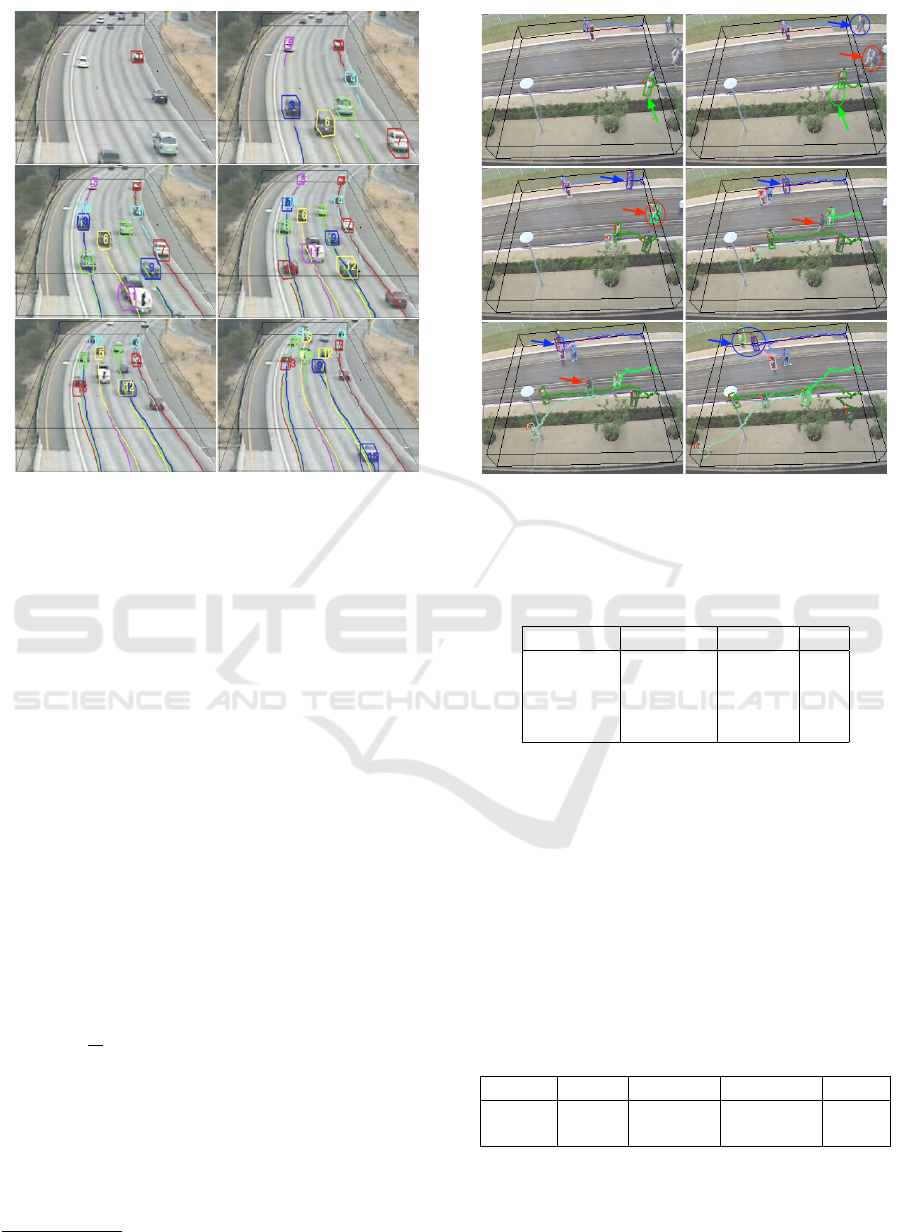
image #1
image #20 image #30
image #40 image #50
image #10
Figure 6: Highway sequence. Thin black lines define the
limits of the 20*100 meters tracking area. Tracked vehicle
estimated cuboids and their past trajectories are overplotted.
at UCSD
3
, captured with a low-resolution (320*240),
low frame rate (10 fps) surveillance webcam, and is
typical of traffic surveillance applications. Figure 6
shows few frames from one of these sequences. On
a second scenery, we track and label multiple pedes-
trians captured with a 640*480, 30 fps IP camera,
downsampled to 320*240 (see figure 7). On both fig-
ures, overplotted thin black lines define the limits of
the tracking area. When entering this area, a new ob-
ject is labeled with a unique identifier, plotted with its
estimated convex hull.
5.3 Multiple Vehicle Tracking
To evaluate the tracker performance, we choose a
short (50 frames) but significant highway sequence,
involving up to 12 vehicles (average number: 9.5)
within a 20x100 meter tracking area. The tracker
performance is measured through an error rate ε =
∑
R
r=1
∑
50
t=1
n
f
n
v
, where n
f
denotes the number of track-
ing failures and n
v
the number of target vehicles, R
is the number of repetitions of the experiment, set
to R = 10, yielding a total number of 4930 vehi-
cle*frame to be tracked. Ground truth has been set
by hand, frame by frame. Table 3 sums up error rate
and frame rate, and shows that the dual proposal filter
MCMC
2
PF clearly outperforms the single proposal
3
http://www.svcl.ucsd.edu/
image # 620 image # 642
image # 717 image # 835
image # 892
image # 935
Figure 7: Pedestrian sequence. Thin black lines define the
limits of the 12x10 meter tracking area. Tracked pedestrian
estimated cuboids and their identity are overplotted.
Table 3: Vehicle tracking failure rate ε and frame rate.
proposal particles error ε fps
single 150 0.27 27
dual 90 0.18 33
single 300 0.18 15
dual 180 0.13 19
on both criteria. For this experiment a constant veloc-
ity model has been used according to table 4 data.
5.4 Multiple Pedestrian Tracking
The tracker performance is assessed as defined in sub-
section 5.3, but over larger sequences (6000 frames).
From 2 to 10 pedestrians are tracked on a 15x12 meter
area. Table 5 results reinforce section 5.3 statements.
Higher frame rate is due to the lower object average
number (4.3 instead of 9.5).
Table 4: Object dynamics.
object σ
p
(m) σ
m
(m/s) σ
a
(rad/s) σ
s
(m)
human 0.4 0.1 0.3 0.05
vehicle 0.75 0.1 0.02 0.1
VISAPP 2009 - International Conference on Computer Vision Theory and Applications
462

Table 5: Pedestrian tracking failure rate ε and frame rate.
proposal particles error ε fps
single 150 0.17 31
dual 90 0.14 37
single 300 0.14 17
dual 180 0.13 19
5.5 Tracking Failures
Losing track of an object: mostly caused by poor
foreground-background segmentation, as illustrated
on figure 7: object target labeled as #6 (green arrow)
in image #620 is lost in image #642 and its estimate
shifts towards a new target. It will be tracked again
at image #717, under a new label: #10. When many
objects are being tracked, the tracker devotes too few
iterations to an entering target, yielding coarse initial-
ization of a new object onto this target, and sometimes
missing it. This is shown on figure 6 by the red vehi-
cle entering bottom right on image #30.
Double tracking of a unique target: on figure 6 im-
age #20 a new vehicle #10 is superimposed onto a
target already tracked by object #3. This error will be
recovered between images #30 and #40.
Single tracking of two targets: on figure 7 image
#642, two pedestrians (blue arrow) will enter while
occluding each other. They are tracked as single ob-
ject #7, and will be recovered at #935, as soon as there
is evidence that two objects are present. This shows
the benefit of the absence of enter location prior. Sim-
ilarly #9 (red arrow) splits #835 (recovery delayed to
image #892 due to poor foreground segmentation).
6 CONCLUSIONS AND FUTURE
WORKS
We have presented a generic multi-object real-time
automatic tracking system, using MCMC Particle Fil-
ter. We have proposed a Multi-Proposal MCMC Par-
ticle Filter (denoted MCMC
P
PF) algorithm, allow-
ing to compute in parallel P proposal likelihoods (the
most computation consuming task), benefitting from
the use of muti-core processing units. We have shown
that dual proposal MCMC
2
PF outperforms single
proposal MCMC
1
PF, improving tracking while re-
quiring less particles, thus yielding higher frame rate.
Our synthetic data experiments allow to generalize
this result to up to 8 parallel proposals, allowing
to look forward to much improved tracking perfor-
mance, especially to track a higher number of ob-
jects, typically 20 to 30 for highway surveillance. The
global likelihood observation function allows to cope
with occlusions and deep scale changes. Though now
only tracking a single object class of objects, the ul-
timate goal of this research is to simultaneously track
and classify several classes of objects, such as road
users, including trucks, cycles and pedestrians, in or-
der to analyze road users interactions. For that pur-
pose, object model selection will be proposed within
the MCMC framework, as a discrete random variable.
REFERENCES
Green, P. J. (1995). Reversible jump markov chain monte
carlo computation and bayesian model determination.
Biometrika, 4(82):711–732.
Isard, M. and MacCormick, J. (2001). Bramble: A bayesian
multiple-blob tracker. In Proc. Int. Conf. Computer
Vision, vol. 2 34-41.
Kanhere, N. K. Pundlik, S. J. and Birchfield, S. T. (2005).
Vehicle segmentation and tracking from a low-angle
off-axis camera. In CVPR, Conference on Com-
puter Vision and Pattern Recognition, volume 2, pages
1152–1157.
Khan, Z., Balch, T., and Dellaert, F. (2005). Mcmc-based
particle filtering for tracking a variable number of in-
teracting targets. IEEE Transactions on Pattern Anal-
ysis and Machine Intelligence, 27:1805 – 1918.
M. Isard and A. Blake (1998). Condensation – conditional
density propagation for visual tracking. IJCV : Inter-
national Journal of Computer Vision, 29(1):5–28.
MacCormick, J. and Blake, A. (1999). A probabilistic ex-
clusion principle for tracking multiple objects. In Int.
Conf. Computer Vision, 572-578.
MacKay, D. (2003). Information Theory, Inference, and
Learning Algorithms. Cambridge University Press.
P. Perez, C. Hue, J. Vermaak, and M. Gangnet (2002).
Color-Based Probabilistic Tracking. In Computer Vi-
sion ECCV 2002, volume 1, pages 661–675.
Smith, K. (2007). Bayesian Methods for Visual Multi-
Object Tracking with Applications to Human Activity
Recognition. PhD thesis, EPFL, Lausanne, Suisse.
Yu, Q., Medioni, G., and Cohen, I. (2007). Multiple target
tracking using spatio-temporal markov chain monte
carlo data association. In IEEE Conference on Com-
puter Vision and Pattern Recognition, pages 1 – 8.
REAL-TIME MULTI-OBJECT TRACKING WITH FEW PARTICLES - A Parallel Extension of MCMC Algorithm
463
