
LESION BOUNDARY SEGMENTATION USING LEVEL SET
METHODS
Elizabeth M. Massey, James A. Lowell
University of Lincoln, Brayford Pool, Lincoln LN6 7TS U.K.
Foster Findlay Associates Limited, Newcastle Technopole Kings Manor, Newcastle Upon Tyne NE1 6PA U.K.
Andrew Hunter, David Steel
University of Lincoln, Brayford Pool, Lincoln LN6 7TS U.K.
Consultant Ophthalmologist, Sunderland Eye Infirmary, Queen Alexandra Road, Sunderland SR2 9HP U.K.
Keywords:
Computer vision, Retinal lesion segmentation, Segmentation, Level set methods.
Abstract:
This paper addresses the issue of accurate lesion segmentation in retinal imagery, using level set methods and
a novel stopping mechanism - an elementary features scheme. Specifically, the curve propagation is guided
by a gradient map built using a combination of histogram equalization and robust statistics. The stopping
mechanism uses elementary features gathered as the curve deforms over time, and then using a lesionness
measure, defined herein, ’looks back in time’ to find the point at which the curve best fits the real object.
We implement the level set using a fast upwind scheme and compare the proposed method against five other
segmentation algorithms performed on 50 randomly selected images of exudates with a database of clinician
marked-up boundaries as ground truth.
1 INTRODUCTION
The diagnosis of diabetic retinopathy is based upon
visually recognizing various clinical features. Retinal
lesions are among the first visual indicators sugges-
tive of diabetic retinopathy. To enable early diagno-
sis, it is therefore necessary to identify both frequency
and position of retinal lesions.
This paper focuses on the segmentation of retinal
lesions and presents an application of level set meth-
ods and a novel elementary features scheme for en-
suring an accurate boundary detection solution. We
present a novel stopping mechanism which uses ele-
mentary features gathered over time as the curve de-
forms and then a calculated lesionness measure to find
the point in time at which the curve best fits the lesion
candidate.
This paper is presented as follows: Sections 2 pro-
vides background information and discusses the cur-
rent literature on region growing schemes as a ba-
sis for comparison. Section 3 describes the level set
method used followed by a description of the algo-
rithm and the process framework. Section 4 discusses
the evaluation results and provides comparison and
observations about the proposed method. Section 5
concludes the paper.
2 PREVIOUS WORK
2.1 Segmentation Algorithms
Retinal exudates are an interesting challenge for seg-
mentation algorithms as they vary in appearance, con-
forming to one of three structures: dot exudates, fluffy
exudates and circumscribed plaques of exudate. Dot
exudates consist of round yellow spots lying superfi-
cially or deep in the sensory retina (Porta and Ban-
dello, 2002). Exudates are usually reflective and may
appear to have a rigid, multifaceted contour, ranging
in color from white to yellow (Chen, 2002).
With varying shapes, sizes, patterns and contrast,
exudate segmentation is a demanding problem, com-
plicated by lighting variation over the image, natural
pigmentation, the intrinsic color of the lesion, and de-
creasing color saturation at lesion boundaries (Gold-
baum et al., 1990).
245
M. Massey E., A. Lowell J., Hunter A. and Steel D.
LESION BOUNDARY SEGMENTATION USING LEVEL SET METHODS.
DOI: 10.5220/0001781402450249
In Proceedings of the Fourth International Conference on Computer Vision Theory and Applications (VISIGRAPP 2009), page
ISBN: 978-989-8111-69-2
Copyright
c
2009 by SCITEPRESS – Science and Technology Publications, Lda. All rights reserved

Several authors have presented algorithms for the
segmentation of exudates in fundus images, attain-
ing varied results. Ward et al., (1989) introduced a
semi-automated exudate detection and measurement
method, in which an operator selected a threshold
value to segment exudates from a shade-corrected
retinal background.
Sinthanayothin et al., (2002) presented a recur-
sive region-growing algorithm applied to a contrast
enhanced image. To reduce the effects of uneven illu-
mination over the fundus, images were pre-processed
to enhance local contrast. The intensity component
of the IHS (Intensity Hue Saturation) model was de-
coupled from color and the fundus images converted
from RGB (Red Green Blue) and normalized to IHS.
Sinthanayothin stated that the algorithm would not
detect faint exudate regions, nor distinguish between
other similar colored lesions.
Wang et al., (2000) defines a feature space F to in-
clude color and exposure information and represents
the red, green and blue (R,G,B) channels as spherical
coordinates. A training set for each of two groupings
is obtained by selecting small sub-windows inside ex-
udate and background regions. The means of each
sub-window are calculated and stored as feature cen-
ters. For each pixel in the fundus image the illumina-
tion and color information are extracted and a mini-
mum distance discriminant is calculated to determine
lesions from background regions.
Osareh et al., (2001) introduced a fuzzy C-Means
clustering algorithm based on the work of (Lim and
Lee, 1990) to segment a color retinal image into ho-
mogeneous regions. To compensate for the wide vari-
ation of color in the fundus, the images are converted
from RGB to IHS, normalized and finally locally con-
trast enhanced (described above in Sinthanayothin et
al., (2002)). Osareh et al., (2001) state that the seg-
mentation by FCM is a conservative process find-
ing all but the faintest (ambiguous) exudate regions.
False positive non-exudate segmented regions were
also found by the algorithm caused by cluster over-
lapping, noise, and uneven color distribution.
Contrast Gradient Region Growing (CG), intro-
duced in (Lowell, 2005), uses a traditional region
growing method employing a pixel intensity aggrega-
tion scheme for region growth, while using a Gaus-
sian smoothed gradient image to iteratively calcu-
late a gradient contrast between a grown (core) inner
boundary and a dilated outer boundary. The algorithm
starts by using a small 5 × 5 sub-window morpholog-
ically applied to the fundus image, and then applying
a maximum filter within each sub-window, producing
peak points. The core region is then grown by ap-
pending (selecting) the brightest neighboring (bound-
ary) pixels on each iteration. This growing process
continues, halting when the grown region loses its
compactness. The final boundary is then located by
using a combination of diameter and contrast to de-
termine the point of growth at which the object’s con-
trast gradient is most significant.
The literature on retinal image object segmenta-
tion using level sets focuses mainly on segmenting
structures rather than pathologies. Excellent work by
Wang et al., (2004) show the power of evolving a
curve to map prominent structures in an image. De-
schampes et al., (2004) used level sets combined with
embedded boundary methods to simulate blood flow
and segment major vessels. Lowell et al., (2004) used
active contours, the fore-runner to level sets, to find
the optic nerve head. The work described herein is
based on the seminal paper from (Osher and Sethian,
1988) and the numerical implementation takes in-
sights from Sapiro, chap. 2, (Sapiro, 2001).
3 LEVEL SET METHOD
For our work in lesion segmentation, level set meth-
ods provide the capability to determine not just the
coarse shape of an object, but are extremely useful
to tease out the fine delicate boundary fissures and
curves that give a deeper look into the overall shape
of a lesion candidate.
3.1 Curve Propagation
Beginning with the definition of level sets from (Os-
her and Sethian, 1988)
φ
t
+ F
|
∇φ
|
= 0, given φ(x,t = 0) (1)
then,
∂φ
∂t
= F
|
∇φ
|
(2)
and
φ
t
+ F
0
|
∇φ
|
+
~
U(x,y,t)
˙
∇φ = εK
|
∇φ
|
(3)
where: φ
t
is the propagating function at time t,
F
0
|
∇φ
|
is the motion of the curve in the direction
normal to the front,
~
U(x, y,t)
˙
∇φ is the term that moves the curve
across the surface,
εK
|
∇φ
|
is the speed term dependent upon curva-
ture.
For our purposes,
~
U(x, y,t)
˙
∇φ is the gradient map, de-
scribed in section 3.3 and εK
|
∇φ
|
is approximated us-
ing a central differencing scheme.
VISAPP 2009 - International Conference on Computer Vision Theory and Applications
246

3.2 Numerical Implementation
We consider curve movement of the form:
∂C
∂t
= β
˜
N (4)
where β = β(k), that is, β is a function of the Eu-
clidean curvature. For simplicity we use β(k) = 1+εk
as our velocity function.
Let φ
n
i
be the value of φ at a point (pixel) i at the
time n. An algorithm to describe the evolution of the
curve over a given time step is
φ
n+1
i j
= φ
n
i j
−4t[max(−β
i j
,0) 4
+
+min(−β
i j
,0)4
−
]
(5)
where u
n
i j
is the ’current’ level set zero, 4t is the time
step (or scaling factor) and the [max...min] describes
the normal component, and where
4
+
= [max(D
−
x
,0)
2
+ min(D
+
x
,0)
2
+ (6)
max(D
−
y
,0)
2
+ min(D
+
y
,0)
2
]
1/2
4
−
= [max(D
+
x
,0)
2
+ min(D
−
x
,0)
2
+ (7)
max(D
+
y
,0)
2
+ min(D
−
y
,0)
2
]
1/2
and D
−
x
,D
+
x
,D
−
y
,D
+
y
are the forward and backward
difference approximations in the x and the y direction,
respectively.
3.3 Gradient Map
The boundary of a lesion can be characterized by the
point of strongest intensity contrast between itself and
the background retina. By determining the gradient of
image I
orig
, this maximum rate of change can be ex-
ploited. Equation 5 propagates the curve φ over the
surface u. Optimally, what we want is to propagate to
an object edge and then stop when the curve has cor-
rectly formed to the (correct) perimeter pixels. To do
this we must provide an edge stopping function. Since
the retinal images are inherently noisy, and the edge
pixels of retinal lesions can look very much like back-
ground pixels, we want a mechanism that smooths
out the noise but preserves the edges. Isotropic fil-
ters (such as Gaussians) smooth the image, but also
lose important detail. Anisotropic filters address the
issue of edge preservation.
Perona and Malik suggested the following edge-
preserving g function (Perona and Malik, 1990)
g(x)x =
2x
2 +
x
2
σ
2
. (8)
The function g(x)x acts as a ‘weighted’ func-
tion in that, small gradient values x will receive high
weight and high gradient values will have low influ-
ence on the diffusion solution. In other words, areas
of high gradient will be ‘smoothed’ less, thus preserv-
ing edges. We applied the function to create our gra-
dient map
g
I
(x,y) =
2 ∗ (I
n
)
(2 − (I
n
)
2
)
(9)
where: I
n
is a histogram equalized, normalized gray-
scale (green channel) image I(x,y) and σ = 1.
3.4 Stopping Criteria
Once the gradient map is generated from the orig-
inal (gray-scale) image the curve propagates for a
given number of iterations. Finding the ‘best’ stop-
ping point for the curve is relative to the object bound-
ary. In cases such as figure 1 the boundary is not
well defined, even with a properly contrasted gradient
map, and especially in the case of bright lesions, the
‘boundary’ can be much the same color as the back-
ground. It is for these reasons that we need to use a
mechanism that is robust to conditions of noise and
illumination variance.
(a) (b)
Figure 1: Curve Fitting: a) Gradient Map b) Match Results.
A traditional use of level sets is to track a curve
to an object’s boundary. In our case, it is more inter-
esting to ‘peek ahead’ by allowing the curve to move
past the optimal boundary and then ‘look back’ and
measure how well-formed the accumulated region is
as a lesion. We define the term lesionness as a com-
bination of compactness (c = p
2
/a), where p is the
perimeter and a is the area (Gonzalez and Woods,
2001) and perimeter size constancy shp and use it as
our ‘stopping’ mechanism. These measurements and
others are explained in detail in section 3.5.2.
3.5 Process and Algorithm
The elementary features algorithm encapsulated in a
three phase framework: 1) Pre-processing 2) Process-
ing and Measurements 3) Best Fit Value Determina-
tion.
LESION BOUNDARY SEGMENTATION USING LEVEL SET METHODS
247
3.5.1 Pre-processing
The single channel, 59x59 pixel image I
orig
is used
to generate a gradient map as discussed in section
3.3. The initial level set begins as a small circle
of radius = 1 and propagates outward according to
equation 5 and as the curve deforms measurements at
each change are taken.
3.5.2 Processing and Measurements
The starting point of the curve is determined using
the simple peak detection algorithm described in Con-
trast Gradient Region Growing (above). The curve
is then allowed to propagate past the optimal point
(boundary) of the object. The purpose of this is to
avoid the underestimation problem inherent in tradi-
tional region growing methods, and take advantage of
‘forward/backward looking’ measures.
We are looking for measurements that can give in-
dicators of how well-formed a region is as a candidate
lesion. Thus, elementary features include 1) the num-
ber of iterations the curve held its perimeter size: shp;
2) the minimum compactness value: c; 3) the number
of iterations the curve held that compactness value:
chp; and 4) the gradient contrast: gc. Using morpho-
logical operations of dilation, equation 10, and ero-
sion, equation 11, two ‘rings’, an inner and an outer
ring, are generated about the curve. The contrast (dif-
ference) between these two rings is calculated.
D = C
0
⊕CE (10)
E = C
0
CE (11)
gc =
∑
p∈D
g
I
(p) −
∑
p∈E
g
I
(p) (12)
where C
0
is the infilled curve, CE is a 3×3 structuring
element, g
I
is the gradient map.
After the curve has moved for a number of iterations
(we use P = 180) it is possible that the curve has
evolved past the optimal point describing the object
boundary. Because of this possibility, the gathered
measurement values are then used to ‘look back in
time’ to find the point at which the curve best fit the
object boundary.
3.5.3 Best Fit Value Determination
Elementary features calculated are: shp,c, chp and
gc. Of these, the two measurements that indicate
curve stabilization (slowing down) are shp and chp.
When the curve reaches an ‘edge’ its propagation rate
slows down and over a number of counted iterations
shp and chp remain constant. We track these stabiliz-
ing points and find that they tend to coincide with the
other important features.
Let q be the iteration number and h(q) be the count
of the number of iterations for which the values of
both chp and shp have held up to and including it-
eration q. Let q
M
, q
N
be the iterations with the two
largest values of h(q), M < N. Let q
c
be the iter-
ation with the smallest value of compactness c, and
q
gc
be the iteration with the largest contrast. Let Z
be the set of critical iterations including q
M
and q
N
,
and q
c
if M ≤ q
c
≤ N, and q
gc
M ≤ q
gc
≤ N. Thus,
the set Z includes the strongest stabilizing points and
any other critical iterations between them. Sometimes
there may be outlying critical iterations. For this rea-
son we determine the largest gap between successive
critical iterations and discarding those after the largest
gap form the set Z
∗
, where Z
∗
⊂ Z. We define the best
fit point, SV , as the average of these critical iterations.
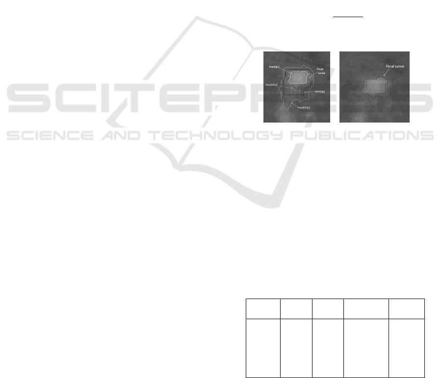
Figure 2 shows the curve plots at the various elemen-
tal values.
SV =
∑
q∈Z
∗
q
#Z
∗
(13)
where #Z
∗
is the number of elements used.
(a) (b)
Figure 2: a) Plots of various elemental points, b) Final
curve.
4 EVALUATION
A comparison is made between the presented algo-
rithm and five segmentation approaches - fuzzy C-
Means clustering, recursive region growing, adap-
tive recursive region growing, contrast gradient region
growing and a color discriminant function. Table 1
shows the results of our evaluation.
Table 1: Algorithm Performance Metrics.
Model Sens. Spec. Accuracy Error
ELS 96.94 98.97 98.87 29.35
CG 96.24 98.71 98.59 36.59
AR 91.13 92.53 92.45 196.15
Fuzzy 88.29 94.18 93.89 158.95
RRG 47.72 90.99 88.85 290.1
DC 64.67 75.77 75.21 644.75
Where:
ELS - Elementary Features Scheme;
VISAPP 2009 - International Conference on Computer Vision Theory and Applications
248

CG - Contrast Gradient;
AR - Adaptive Recursive;
Fuzzy - Fuzzy C-means;
RRG - Recursive Region Grow;
DC - Color Discriminant.
All algorithms were implemented and evaluated
against a reference standard dataset of 50 randomly
selected lesion images. Each image is provided with
boundary markups by an expert ophthalmologist us-
ing custom designed software. The images are pro-
vided by the Sunderland Eye Infirmary with permis-
sion to be used in this research.
The benchmark comparison with the aforemen-
tioned techniques was achieved by measuring the
number of common pixels shared between the ref-
erence standard and the algorithm’s segmented area.
The values in Table 1 were measured using pixel-wise
sensitivity, specificity, accuracy and error-rate.
5 CONCLUSIONS
Algorithms for the automated segmentation and clas-
sification of candidate lesions have been presented.
Although a number of algorithms have been pub-
lished for lesion segmentation, many are unreliable
due to marginal color and intensity difference be-
tween diabetic lesions and the background retina.
This limited contrast has an adverse effect on alternate
algorithms causing poor lesion boundary estimations.
Experimental comparisons have been conducted
on five segmentation approaches - Contrast Gradient,
Fuzzy C-Means clustering, recursive region grow-
ing, adaptive recursive region growing, and a color
discriminant function. All algorithms were evalu-
ated against a randomly-selected image set with oph-
thalmic lesion boundary demarcation. The results
shown in Section 4 demonstrate the advantage of al-
lowing the curve propagation (region growing) to run
past the optimal boundary point, thus providing a
‘peek ahead’ to adjacent areas. Then using gathered
elementary features to ‘look back in time’ to deter-
mine the best fitting curve.
REFERENCES
Chen, H.-C. (2002). Vascular Complications of Diabetes;
current issues in pathogenesis and treatment, chap-
ter 10, pages 97–108. Blackwell Publishing.
Deschamps, T., Schwartz, P., Trebotich, D., Colella, P., Sa-
loner, D., and Malladi, R. (2004). Vessel segmenta-
tion and blood flow simulation using level-sets and
embedded boundary methods. Computer Assisted Ra-
diology and Surgery. Proceedings of the 18th Interna-
tional Congress and Exhibition, 1268:75–80.
Goldbaum, M., Katz, N., Nelson, M., and Haff, L. (1990).
The discrimination of similarly colored objects in
computer images of the ocular fundus. Investigative
Ophthalmology & Visual Science, 31:617–623.
Gonzalez, R. C. and Woods, R. E. (2001). Digital Image
Processing. Prentice Hall, Upper Saddle River, NJ.
Lim, Y. W. and Lee, S. U. (1990). On the color image
segmentation algorithm based on the thresholding and
the fuzzy c-means technique. Pattern Recognition,
23:935–952.
Lowell, J. (2005). Automated Retinal Analysis. PhD thesis,
University of Durham.
Lowell, J., Hunter, A., Steel, D., Basu, A., Ryder, R.,
Fletcher, E., and Kennedy, L. (2004). Optic nerve
head segmentation. IEEE Transactions on Medical
Imaging, 23(2):256–264.
Osareh, A., Mirmehdi, M., Thomas, B., and Markham, R.
(2001). Automatic recognition of exudative macu-
lopathy using fuzzy c-means clustering and neural net-
works. In Claridge, E. and Bamber, J., editors, Medi-
cal Image Understanding and Analysis, pages 49–52.
BMVA Press.
Osher, S. and Sethian, J. A. (1988). Fronts propagating
with curvature-dependent speed: Algorithms based on
Hamilton-Jacobi formulations. Journal of Computa-
tional Physics, 79:12–49.
Perona, P. and Malik, J. (1990). Scale-space and edge de-
tection using anisotropic diffusion. IEEE Transac-
tions on Pattern Analysis and Machine Intelligence,
12(7):629–639.
Porta, M. and Bandello, F. (2002). Diabetic retinopathy a
clinical update. Diabetologia, 45(12):1617–1634.
Sapiro, G. (2001). Geometric Partial Differential Equations
and Image Analysis. Cambridge University Press.
Sinthanayothin, C., Boyce, J., Williamson, T., Cook, H.,
Mensah, E., and Lal, S. andUsher, D. (2002). Auto-
mated detection of diabetic retinopathy on digital fun-
dus images. Diabetic Medicine, 19:105–112.
Wang, H., Hsu, W., Goh, K., and Lee, M. (2000). An effec-
tive approach to detect lesions in color retinal images.
In Proceedings IEEE Conference on Computer Vision
and Pattern Recognition, volume 2, pages 181–186.
Wang, L., Bhalerao, A., and Wilson, R. (2004). Robust
modelling of local image structures and its application
to medical imagery. In ICPR04, pages III: 534–537.
Ward, N., Tomlinson, S., and Taylor, C. J. (1989). Im-
age analysis of fundus photographs: the detection
and measurement of exudates associated with diabetic
retinopathy. Ophthalmology, 96(1):80–86.
LESION BOUNDARY SEGMENTATION USING LEVEL SET METHODS
249
