GEOMETRY CLOSURE FOR HEMODYNAMICS SIMULATIONS
J. Bruijns
Philips Research, High Tech Campus 36, 5656 AE, Eindhoven, The Netherlands
R. Hermans
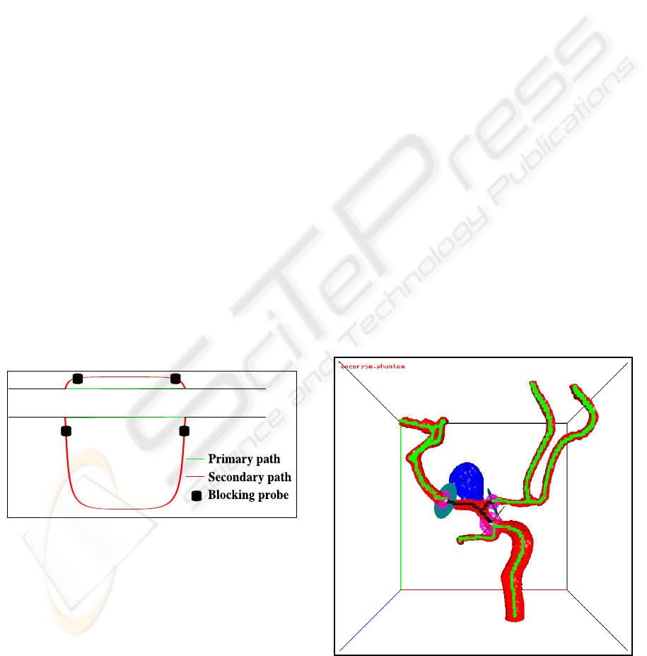
Philips Healthcare, Veenpluis 8, 5684 PC, Best, The Netherlands
Keywords:
3D rotational angiography, Computer assisted diagnosis, Hemodynamics simulations.
Abstract:
Physicians may treat an aneurysm by injecting coils through a catheter into the aneurysm, or by anchoring
a stent as a flow diverter. Since such an intervention is risky, a patient is only treated when the probability
of aneurysm rupture is relatively high. Hemodynamic properties of aneurysmal blood flow, extracted by
computational fluid dynamics calculations, are hypothesized to be relevant for predicting this rupture. Since
hemodynamics simulations require a closed vessel section with defined inflow and outflow points, and since
the user can easily overlook small side branches, we have developed an algorithm for fully-automatic geometry
closure of an open vessel section. Since X-ray based flow returns an indication for the needed length to have a
developed flow inside the geometry, we have also developed an algorithm to create a geometry closure around
an aneurysm based on a length criterion. After both geometry closure algorithms were tested elaborately,
practicability of the hemodynamics workstation is currently being tested.
1 INTRODUCTION
Volume representations of blood vessels acquired by
3D rotational angiography after injection with a con-
trast agent (Moret et al., 1998) have a clear distinc-
tion in gray values between tissue and vessel voxels.
Therefore, these volume representations are very suit-
able for diagnosing an aneurysm, a local widening of
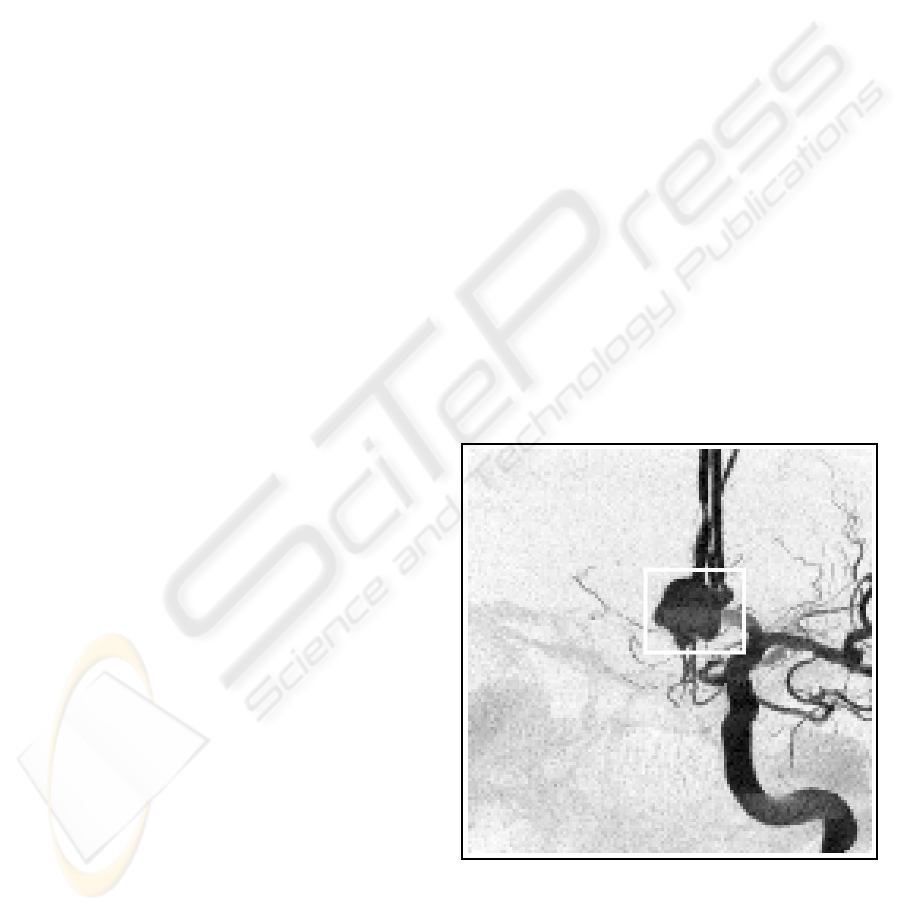
a vessel caused by a weak vessel wall (see Figure 1).
Physicians may treat an aneurysm by first mov-
ing a catheter inside the aneurysm and next injecting
coils through the catheter into the aneurysm. An al-
ternative that is becoming increasingly popular is us-
ing a stent as a flow diverter. Since such an interven-
tion is risky, a patient is only treated when the prob-
ability of aneurysm rupture is relatively high. So, it
is very important to be able to estimate the probabil-
ity of aneurysm rupture (see also www.aneurist.org).
Hemodynamic properties of aneurysmal blood flow
are hypothesized to be relevant for predicting this rup-
ture.
Since hemodynamics simulations (i.e. computa-
tional fluid dynamics calculations using for example
finite element methods) gives highly detailed results
in space and time of wall shear stress, pressure, flow
Figure 1: An aneurysm inside the white rectangle.
impact regions, vorticity and “turbulent” flow, hemo-
dynamics simulations can be used to assess the risk
of an aneurysm rupture (Butty et al., 2002; Venugopal
et al., 2005; Cebral et al., 2005; Castro et al., 2005).
The points where blood is flowing into the ge-
154
Bruijns J. and Hermans R. (2009).
GEOMETRY CLOSURE FOR HEMODYNAMICS SIMULATIONS.
In Proceedings of the Fourth International Conference on Computer Vision Theory and Applications, pages 153-161
DOI: 10.5220/0001782701530161
Copyright
c
SciTePress
ometry and out of the geometry can be selected by
the user or derived from X-ray based flow (Waechter
et al., 2008). The user may not have selected all
points needed to close the geometry; therefore, we
have developed an algorithm for fully-automatic ge-
ometry closure of an open vessel section. The basic
hypothesis of our algorithm is that the vessel branches
on the shortest paths between the selected points are
members of the flow section. Connections between
these member branches and the other vessel branches
which are not marked by the user as either an inflow
or an outflow point (i.e. unintentional open connec-
tions), are closed by a blockade (further details are
given in Section 4).
X-ray based flow returns amongst other things an
indication for the needed length to have a developed
flow inside the geometry. Therefore, we have devel-
oped also an algorithm to create a geometry closure
around an aneurysm based on a length criterion. First,
a blockade is created at those points of the vessel
branches for which the shortest path distance to the
aneurysm is equal to this length. In a second step, a
blockade is created at those extremities of the vessels
for which the shortest path distance to the aneurysm
is less than this length (described in Section 5).
We have used 48 clinical volume datasets with an
aneurysm to test both geometry closure algorithms
elaborately (reported in Section 7).
2 RELATED WORK
In 2006 the European funded Aneurist project was
started (www.aneurist.org). This project has the goal
to provide an integrated decision support system to as-
sess the risk of cerebral aneurysm rupture in patients
and to optimize their treatments. Hemodynamics sim-
ulations on patient specific aneurysm is a part of this.
Hemodynamics simulations is a topic of increas-
ing interest. Major advances towards clinical rele-
vance and applicability have been made by dr. J. Ce-
bral of the department of computational and data sci-
ences of George Mason University, USA, VA.
Advances in flow assessment directly from the X-
ray images has been made in the work of I. Waechter
(Waechter et al., 2008).
3 PREAMBLE
Our starting point is a segmented volume with tissue
voxels, aneurysm voxels and “normal” vessel voxels
(Bruijns et al., 2007), and the set of directed graphs
(one for each component of the voxel vessel struc-
tures) with nodes (one for each vessel junction, one
for each vessel extremity and one for each aneurysm
neck; nodes at the aneurysm necks are called “neck
nodes”) and skeleton branches (one for each vessel
branch) (Bruijns, 2001). A skeleton branch consists
of a set of face connected vessel voxels, called “skele-
ton voxels”. The skeleton voxels, located close to the
center line of the vessel branch, have a unique label
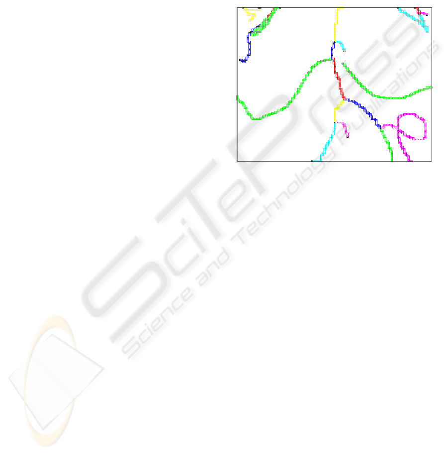
per vessel branch. An example is shown in Figure 2.
Figure 2: The skeleton voxels of the graphs.
The skeleton voxels are displayed in a color ac-
cording to their label but skeleton voxels with differ-
ent labels can have the same color because of the lim-
ited number of colors used for display.
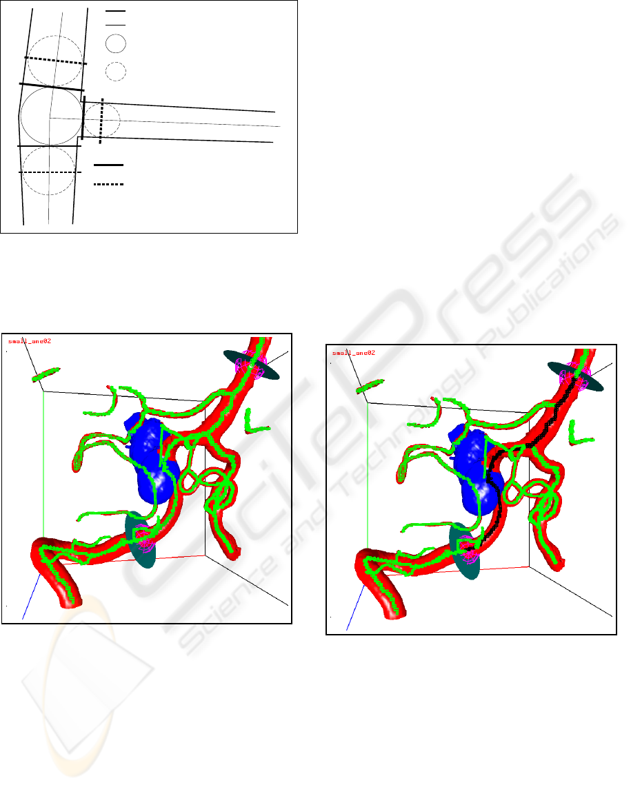
The nodes are equipped with geometry (see Fig-
ure 3). A center sphere together with the center planes
give the position, the size and the delineation of the
center region (i.e. the junction). The branch spheres
together with the branch planes give the size and the
direction of the branch regions adjacent to the center
region.
4 FULLY-AUTOMATIC
GEOMETRY CLOSURE OF AN
OPEN VESSEL SECTION
Hemodynamics simulations are only possible when
all points where blood is flowing into the geometry
and out of the geometry are known. The user can
select the vessel section (called “flow section” from
now on) by launching a series of probes (Bruijns et al.,
2005) on to the vessel branches (see Figure 4). The
plane of such a boundary probe separates the vessel
voxels at one side of the plane from the vessel vox-
els at the other side of the plane. If the normal of
this plane is pointing into the intended flow section,
GEOMETRY CLOSURE FOR HEMODYNAMICS SIMULATIONS
155
vessel boundary
direction lines
center sphere
branch sphere
center planes
branch planes
Figure 3: The node geometry.
the vessel voxels at the positive side of the plane are
members of the flow section and the vessel voxels at
the negative side not.
Figure 4: Initial boundary probes; the skeleton voxels are
green; the aneurysm part is blue.
Our program connects each boundary probe to a
skeleton voxel. The corresponding skeleton voxel is
called a “boundary skeleton voxel”. Since the closure
of a flow section can be checked more easily when a
boundary skeleton voxel has exactly two face neigh-
bor skeleton voxels (will be given further detail in
Section 6), and since the first and last skeleton voxel
of a skeleton branch has either one or more than two
face neighbor skeleton voxels, boundary probes are
connected to a skeleton voxel between the first and
last skeleton voxel of a skeleton branch (changing the
position of the probe slightly if necessary).
Since the user can easily forget small side
branches, a possible open flow section (i.e. a flow
section with not all skeleton branches delimited by
a probe as shown in Figure 4) can be closed fully-
automatically by the following algorithm:
1. Mark all skeleton voxels of the shortest paths,
possibly through the aneurysm, between each pair
of boundary probes as member of the flow section.
The algorithm to compute the shortest path
through the aneurysm is similar as the algorithm
to compute the path for a connection tube (Bruijns
et al., 2005).
The basic hypothesis of our algorithm is that the
skeleton voxels on the shortest paths are members
of the flow section. Figure 5 is an example. The
black skeleton voxels are located on the shortest
paths and thus members of the flow section, the
green skeleton voxels are not (yet) members of the
flow section. Note that some of the green skeleton
voxels are located in the intended flow section.
Figure 5: The skeleton voxels of the shortest paths are
black, the other skeleton voxels are green.
2. Mark the open vessel nodes type 1.
After the first step the nodes, located on the short-
est paths, have at least one skeleton branch from
which the skeleton voxel closest to this node
is a member of the flow section (such a skele-
ton branch is called a “member branch” for this
node). If such a node has also a skeleton branch
from which the skeleton voxel closest to this node
is not a member of the flow section (such a skele-
ton branch is called a “non-member branch” for
this node), the flow section is open along that
VISAPP 2009 - International Conference on Computer Vision Theory and Applications
156
skeleton branch (i.e. there is no boundary probe
between a member skeleton voxel and a non-
member skeleton voxel).
In some cases, a neck node (see Section 3), not
located on the shortest paths, is connected via a
very short skeleton branch to an open vessel node
type 1 (i.e. the center spheres of the two nodes
overlap). In such a case, the aneurysm borders on
the flow section. Therefore, such a neck node is
also marked as an open vessel node type 1, and
the skeleton voxels of the short skeleton branch
are marked as member of the flow section. Af-
ter this procedure, one or both nodes may be no
longer an open vessel node type 1 (i.e. all its
skeleton branches are member branches), but that
is taken care of during the creation of extra bound-
ary probes further on.
3. Mark the open vessel nodes type 2.
If a neck node is a member of the flow sec-
tion, there will be no boundary probe between
the intended flow section and the aneurysm: the
aneurysm is member of the intended flow section
(i.e. the skeleton voxels of the neck nodes are con-
ceptually face connected via the aneurysm). In
this case, boundary probes are required around the
neck nodes which are not located on the shortest
paths, to close the flow section.
4. Create and launch boundary probes on the non-
member branches of the open vessel nodes type 1,
just outside the center sphere. Mark all skeleton
voxels along the non-member branches between
open vessel nodes type 1 and the corresponding
boundary probe as member of the flow section.
Since the new boundary probe is placed just out-
side the center sphere of the current node, the
skeleton voxels and thus the neighbor vessel vox-
els, located in the flow section, become members
of the flow section.
Examples of extra boundary probes are shown in
Figure 6. Comparing Figure 5 with Figure 6 re-
veals the extra black skeleton voxels on the skele-
ton branches which are now also members of the
flow section.
5. Create and launch boundary probes on the skele-
ton branches of the open vessel nodes type 2, as
close as possible to the node.
Since all skeleton branches of an open vessel
node type 2 are not members of the flow section,
boundary probes has to be placed on each skele-
ton branch so that the hemodynamics simulations
cannot “escape” through the aneurysm to other
vessel parts.
Figure 6: The closed flow section. The skeleton voxels
of the flow section are black, the other skeleton voxels are
green.
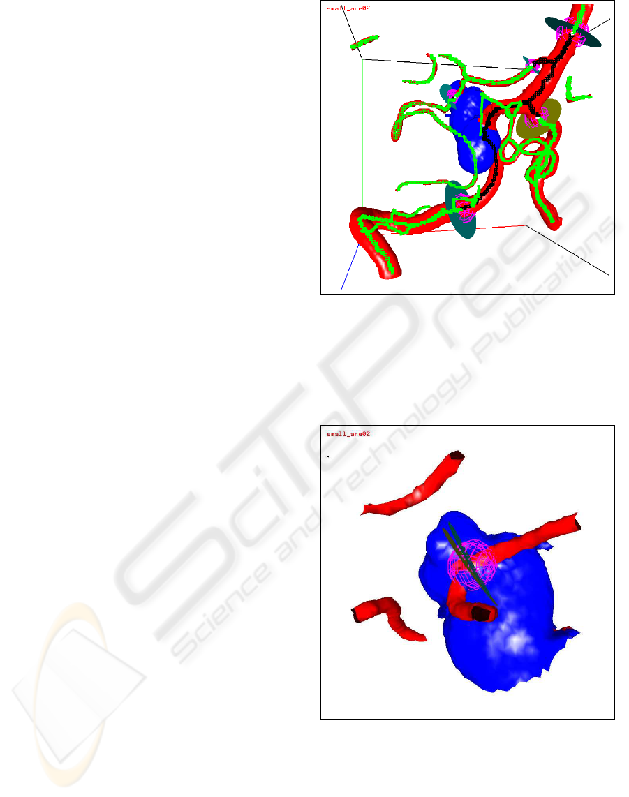
Examples of such boundary probes are shown in
Figure 6 at the top of the aneurysm, and more
clearly in Figure 7.
Figure 7: The boundary probes at a neck, not on the shortest
paths.
Remarks:
1. The initial boundary probes are created by the
user either as inflow or as outflow probes. The ex-
tra boundary probes are created by our algorithm
as blocking probes. Afterwards, the user can mark
GEOMETRY CLOSURE FOR HEMODYNAMICS SIMULATIONS
157
the extra boundary probes as an inflow or an out-
flow probe. After the user has finished possible
adjustments, the vessel is completely closed at
the remaining blocking probes by an extra surface
mesh.
2. In some cases two open vessel nodes type 1 are
connected by a very short non-member branch.
In this case, no extra boundary probes are cre-
ated and all skeleton voxels of such a branch are
marked as members of the flow section.
3. In some cases two open vessel nodes type 1 are
connected by two paths (i.e. there is a cycle
in the vessel graph as shown in Figure 8). Our
algorithm selects only the shortest of these two
paths (called the “primary path”). The other path
(called the “secondary path”) will be blocked by
two blocking probes at the begin and at the end
of this path. If the user wants to include also the
secondary path and if this secondary path is only
slightly longer than the primary path (top case in
Figure 8), application of our algorithm to the ex-
tended probe configuration (i.e. the extra block-
ing probes become now initial boundary probes)
will include the secondary path because the short-
est path between the two blocking probes will run
along the secondary path. If the secondary path is
too long (i.e. if the shortest path between the two
blocking probes runs also along on the primary
path; bottom case of Figure 8) the secondary path
can be included by launching an extra probe on to
the secondary path.
Figure 8: Geometry closure for two cycle cases.
5 FULLY-AUTOMATIC
GEOMETRY CLOSURE OF AN
ANEURYSM
X-ray based flow helps to estimate amongst other
things an indication for the needed length to have a
developed flow inside the geometry (Waechter et al.,
2008). Therefore, we have developed an algorithm to
create a geometry closure around an aneurysm based
on a length criterion (i.e. a path distance in face con-
nected voxels). This algorithm consists of the follow-
ing steps:
1. Compute for each node the shortest path distance
to the aneurysm (i.e. to the closest neck node).
2. Launch a blocking probe to each skeleton branch
for which the path distance of one node is less than
or equal to the needed length and the path distance
of the other node is greater than the needed length.
Traveling along this skeleton branch, the probe is
connected to the first skeleton voxel for which the
path distance is greater than or equal to the needed
length. Since a boundary skeleton voxel should be
located between the first and last skeleton voxel
of a skeleton branch, the second skeleton voxel is
used when the first skeleton voxel fulfills the dis-
tance condition, and the last but one is used when
the last skeleton voxel fulfills the distance condi-
tion.
3. Launch a blocking probe to each skeleton branch
for which one node is an extremity node with
a path distance less than or equal to the needed
length. The second skeleton voxel counted from
the extremity node is used as boundary skeleton
voxel.
An example of a small flow section around an
aneurysm is shown in Figure 9 and of a large flow
section in Figure 10.
Figure 9: A small flow section around an aneurysm. The
skeleton voxels of the flow section are black, the other
skeleton voxels are green.
VISAPP 2009 - International Conference on Computer Vision Theory and Applications
158
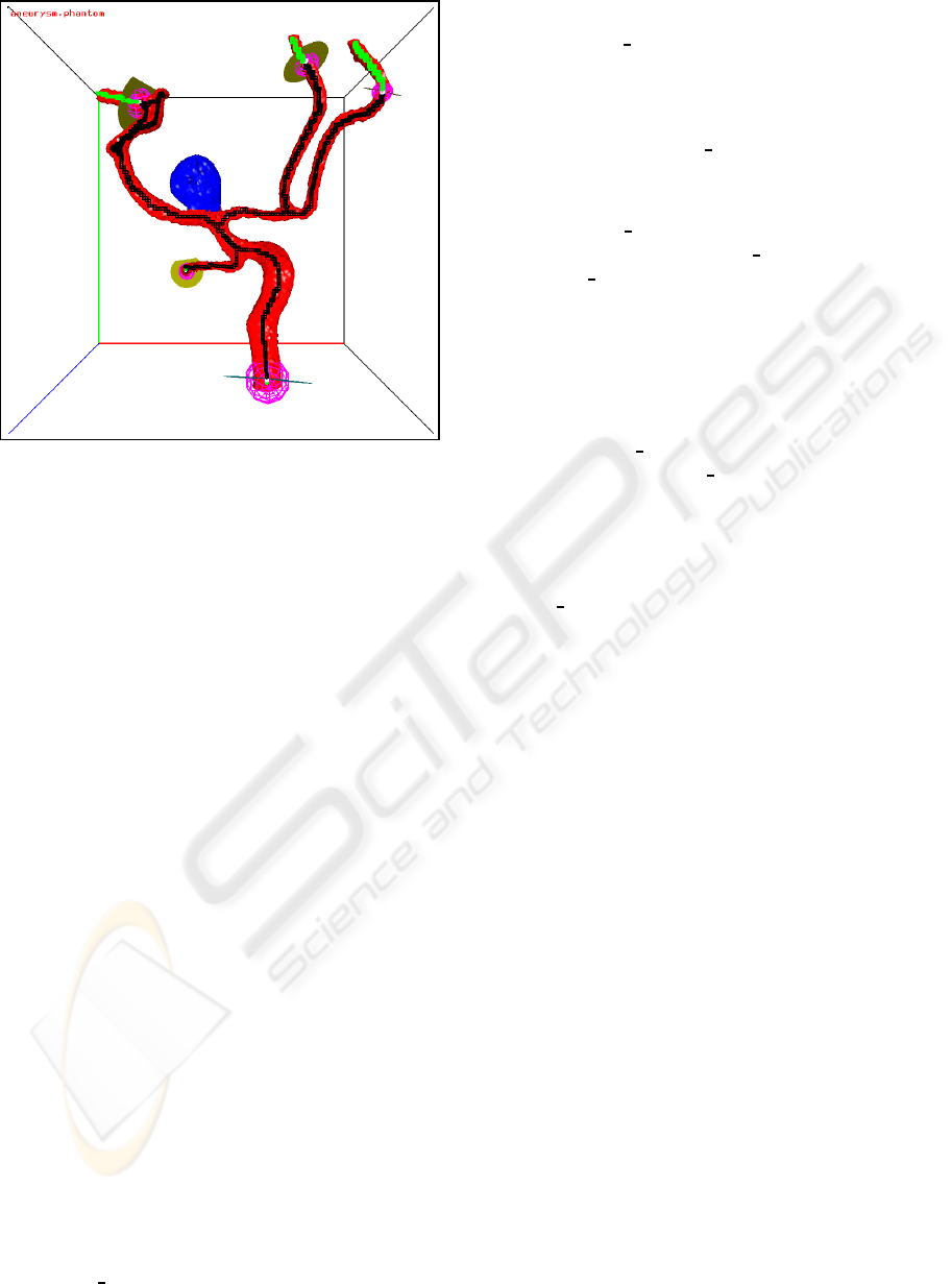
Figure 10: A large flow section around an aneurysm. The
skeleton voxels of the flow section are black, the other
skeleton voxels are green.
Remark:
In some cases, small side branches should be ig-
nored in the hemodynamics simulations. In that case,
this algorithm should be adapted. It may be done as
follows. Instead of pure path distances a kind of path
expenses should be used. These path expenses are the
accumulated branch expenses along the “minimum”
path. The branch expenses of small side branches
(e.g. diameter less than a user defined value) are set
to a very high value. The branch expenses of the other
branches are set to the path distance of the branch.
6 VERIFICATION
6.1 Detection of an Open Flow Section
As already mentioned in Section 4, the boundary
skeleton voxels to which the boundary probes are
launched, are located between the first and last skele-
ton voxel of a skeleton branch. So, each boundary
skeleton voxel has exactly two face neighbor skele-
ton voxels, one located at the positive side and one
located at the negative side of the probe’s plane. The
closure of the flow section will be verified by looking
at the membership of these two face neighbor skele-
ton voxels. The membership of a skeleton voxel can
be computed by the following labelling algorithm:
1. Mark all skeleton voxels with the label
“FLOW IN”, indicating that they are as yet
member of the flow section.
2. Mark the boundary skeleton voxels with the la-
bel “FLOW BLOCK”, indicating that labelling
should not be continued across this skeleton
voxel.
3. Mark all skeleton voxels at the extremity nodes
with the label “FLOW OUT”, indicating that they
are not member of the flow section.
4. Mark all skeleton voxels, labelled with the la-
bel “FLOW IN”, face connected to a skeleton
voxel with the label “FLOW OUT”, with the label
“FLOW OUT”, indicating that they are no longer
member of the flow section. This step is repeated
until no skeleton voxels are changed anymore.
As mentioned in Section 4, the skeleton voxels of
the neck nodes are conceptually face connected
via the aneurysm. Therefore, if one of the neck
nodes (i.e. its skeleton voxel) is marked with the
label “FLOW OUT”, all neck nodes are marked
with the label “FLOW OUT”.
A possible open flow section is detected by com-
paring the face neighborskeleton voxels of the bound-
ary skeleton voxels. A flow section is open if and only
if both face neighbor skeleton voxels have the label
“FLOW OUT”, indicating that both skeleton voxels
are not a member of the flow section.
Remarks:
1. This verification procedure is used both for check-
ing whether the geometry closure algorithm de-
scribed in Section 4 has to be executed and for
checking whether the selected geometry closure
algorithm (i.e. the one described in Section 4 or
the one described in Section 5) resulted in a closed
flow section.
2. After the labelling algorithm is finished, possible
internal probes are removed (just before check-
ing whether the flow section is open or closed).
An internal probe is a probe for which both face
neighbor skeleton voxels are member of the flow
section. An example of a set of initial boundary
probes with one internal probe is shown in Fig-
ure 11. The closed flow section is shown in Fig-
ure 12. The final flow section with the internal
probe removed is shown in Figure 13.
6.2 Detection of Multiple Flow Sections
After possible internal probes have been removed and
the geometry closure of the flow section has been ver-
ified, verification of the number of components of the
flow section can be performed. After all, for hemody-
namics simulations the flow section should consist of
a single connected component.
GEOMETRY CLOSURE FOR HEMODYNAMICS SIMULATIONS
159
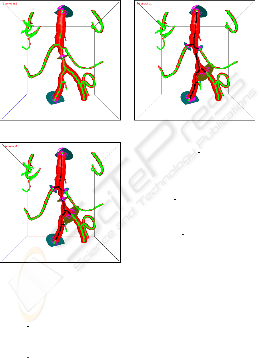
Figure 11: Initial boundary probes with one internal probe.
The skeleton voxels are green.
Figure 12: The closed flow section for the internal probe
case. The skeleton voxels of the flow section are black, the
other skeleton voxels are green.
Checking whether the flow section consists of a
single connected component is also performed by a
labelling algorithm:
1. Mark all boundary skeleton voxels with the label
“FLOW IN”.
2. Mark the first boundary skeleton voxel with the
label “FLOW FIRST”.
3. Mark all skeleton voxels, labelled with the label
“FLOW IN”, face connected to a skeleton voxel
Figure 13: The flow section with the internal probe re-
moved. The skeleton voxels of the flow section are black,
the other skeleton voxels are green.
with the label “FLOW FIRST”, with the label
“FLOW FIRST”. This step is repeated until no
skeleton voxels are changed anymore.
As mentioned in Section 4, the skeleton voxels of
the neck nodes are conceptually face connected
via the aneurysm. Therefore, if one of the neck
nodes (i.e. its skeleton voxel) is marked with the
label “FLOW FIRST”, all neck nodes are marked
with the label “FLOW FIRST”. So, two flow sec-
tions connected to an aneurysm are considered a
single connected component.
4. Check whether all boundary skeleton voxels have
the label “FLOW FIRST”.
If so, the flow section consist of a single connected
component.
An example of two separated closed flow sections
is shown in Figure 14.
7 EXPERIMENTS AND RESULTS
7.1 For Geometry Closure of an
Aneurysm
We have applied the method for fully-automatic ge-
ometry closure of an aneurysm (see Section 5) to
48 clinical volume datasets with an aneurysm (15
of them with a resolution of 256x256x256 voxels,
the rest 128x128x128 voxels), acquired with the 3D
Integris system (Philips-Medical-Systems-Nederland,
VISAPP 2009 - International Conference on Computer Vision Theory and Applications
160
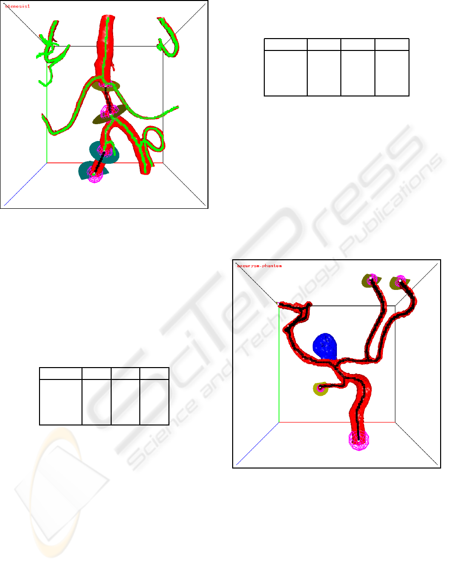
Figure 14: Two separated closed flow sections. The skele-
ton voxels of the flow sections are black, the other skeleton
voxels are green.
2001). The voxel size varies between 0.2 and 1.2 mil-
limeter. We have tested three lengths (path distances
in face connected voxels): 31, 101 and 171. Examples
are shown in Figure 9 and Figure 10.
Table 1: The characteristics of the number of blocking
probes, created by fully-automatic geometry closure of 48
aneurysms, for three different lengths (i.e. path distances in
face connected voxels).
Length: 31 101 171
min. 2.0 2.0 3.0
median 4.0 8.0 11.5
mean 4.3 9.1 13.7
max. 11.0 24.0 36.0
The characteristics of the number of blocking
probes, created by fully-automatic geometry closure
of 48 aneurysms, for these three lengths, are given in
Table 1. The characteristics of the elapsed times in
seconds are given in Table 2. The elapsed times for
the 256x256x256 volumes are divided by 2 to com-
pensate for the on average two times longer path dis-
tances. As is clear from this table, the elapsed times
are increasing for larger lengths.
After the blocking probes are created, the flow
section is checked with the verification algorithms,
described in Section 6. For all cases, the flow section
was a single connected closed flow section.
Table 2: The characteristics of the elapsed times in seconds
for fully-automatic geometry closure of 48 aneurysms, for
three different lengths.
Length: 31 101 171
min. 0.016 0.020 0.024
median 0.052 0.103 0.163
mean 0.064 0.119 0.173
max. 0.200 0.304 0.416
7.2 For Closure of an Open Flow
Section
We have applied the method for fully-automatic ge-
ometry closure of an aneurysm also to generate tests
for geometry closure of an open flow section (see Sec-
tion 4). Indeed, if the required length is set to a very
large number, blocking probes will be generated at the
extremity nodes of the vessel graph(s) connected to
the aneurysm. An example of the generated extremity
probes is shown in Figure 15.
Figure 15: The extremity probes.
We have used each pair of the generated extrem-
ity probes as initial boundary probes. An example of
the generated blocking probes for two of the initial
boundary probes is shown in Figure 16.
The characteristics of the number of extremity
probes NE, the number of tests NT (i.e. the number
of pairs of initial boundary probes) and the resulting
number of blocking probes NB including the two ini-
tial probes are given in Table 3. The total number of
test was 11869. For all tests, the flow section was a
single connected closed flow section.
GEOMETRY CLOSURE FOR HEMODYNAMICS SIMULATIONS
161
Figure 16: The closed flow section for probes 1 and 3.
The skeleton voxels of the flow section are black, the other
skeleton voxels are green.
Table 3: The characteristics of the number of extremity
probes NE, the number of tests NT and the resulting num-
ber of blocking probes NB including the two initial probes
for fully-automatic geometry closure of 11869 open flow
sections
NE NT NB
min. 3.0 3.0 3.0
median 15.5 112.5 14.0
mean 19.2 247.3 14.8
max. 56.0 1540.0 48.0
8 CONCLUSIONS
The following conclusions can be drawn from the re-
sults, the figures and the experiences gathered during
testing:
1. Fully-automatic geometry closure of an aneurysm
gives always correct (i.e. a single connected
closed flow section) and visually acceptable re-
sults.
2. Fully-automatic geometry closure of an open flow
section gives correct and visually acceptable re-
sults except when multiple closed flow sections
arise from the initial boundary probes.
3. Preparing patient specific geometries for compu-
tational fluid dynamics is a time-consuming and
error-prone task. The work above is the first to au-
tomatically create and validate an error free closed
simulation domain. It has been implemented in
a simulation and visualization software environ-
ment that allows a user to prepare a simulation in
a matter of minutes instead of an hour of work.
4. Whether flow sections, generated by fully-
automatic geometry closure of an aneurysm based
on a length criterion, are suitable for hemodynam-
ics simulations has yet to be investigated.
REFERENCES
Bruijns, J. (2001). Fully-automatic branch labelling of
voxel vessel structures. In Proc. VMV, pages 341–350,
Stuttgart, Germany.
Bruijns, J., Peters, F., Berretty, R., and Barenbrug, B.
(2007). Fully-automatic correction of the erroneous
border areas of an aneurysm. In Proc. BVM, pages
293–297, Muenchen, Germany.
Bruijns, J., Peters, F., Berretty, R., van Overveld, C., and ter
Haar Romeny, B. (2005). Computer-aided treatment
planning of an aneurysm: The connection tube and the
neck outline. In Proc. VMV, pages 265–272, Erlangen,
Germany.
Butty, V., Gudjonsson, K., P.Buchel, Makhijani, V., Ven-
tikosa, Y., and D.Poulikakos (2002). Residence times
and basins of attraction for a realistic right inter-
nal carotid artery with two aneurysms. Biorheology,
39:387–393.
Castro, M., Putman, C., and Cebral, J. (2005). Computa-
tional modeling of cerebral aneurysms in arterial net-
works reconstructed from multiple 3d rotational an-
giography images. In Proc. SPIE: Medical Imaging,
volume 5746, pages 233–244, San Diego, CA, USA.
Cebral, J., Castro, M., Millan, D., Frangi, A., and Putman,
C. (2005). Pilot clinical investigation of aneurysm
rupture using image-based computational fluid dy-
namics models. In Proc. SPIE: Medical Imaging, vol-
ume 5746, pages 245–256, San Diego, CA, USA.
Moret, J., Kemkers, R., de Beek, J. O., Koppe, R., Klotz,
E., and Grass, M. (1998). 3D rotational angiography:
Clinical value in endovascular treatment. Medica-
mundi, 42(3):8–14.
Philips-Medical-Systems-Nederland (2001). INTEGRIS
3D-RA. instructions for use. release 2.2. Techni-
cal Report 9896 001 32943, Philips Medical Systems
Nederland, Best, The Netherlands.
Venugopal, P., Duckwiler, G., Valentino, D., Chen, H.,
Villablance, P., Vinuela, F., Kemkers, R., and Haas,
H. (2005). Correlating aneurysm growth to hemody-
namic parameters: the case of a patient-specific ante-
rior communicating artery aneurysm. In Proc. SPIE:
Medical Imaging, volume 5746, pages 780–791, San
Diego, CA, USA.
Waechter, I., Bredno, J., Hermans, R., Weese, J., Barratt, D.,
and Hawkes, D. (2008). Evaluation of model-based
blood flow quantification from rotational angiography.
In Proc. SPIE: Medical Imaging, volume 6916, San
Diego, CA, USA.
VISAPP 2009 - International Conference on Computer Vision Theory and Applications
162
