INCREMENTAL MACHINE LEARNING APPROACH FOR
COMPONENT-BASED RECOGNITION
Osman Hassab Elgawi
Image Science and Engineering Laboratory, Tokyo Institute of Technology, Tokyo, Japan
Keywords:
Random forests (RFs), Object recognition, Histograms, Covariance descriptor.
Abstract:
This study proposes an on-line machine learning approach for object recognition, where new images are
continuously added and the recognition decision is made without delay. Random forest (RF) classifier has
been extensively used as a generative model for classification and regression applications. We extend this
technique for the task of building incremental component-based detector. First we employ object descriptor
model based on bag of covariance matrices, to represent an object region then run our on-line RF learner to
select object descriptors and to learn an object classifier. Experiments of the object recognition are provided to
verify the effectiveness of the proposed approach. Results demonstrate that the propose model yields in object
recognition performance comparable to the benchmark standard RF, AdaBoost, and SVM classifiers.
1 INTRODUCTION
Object recognition is one of the core problems in
computer vision, and it turns out to be extremely diffi-
cult for reproducing in artificial devices, simulated or
real. Specifically, an object recognition system must
be able to detect the presence or absence of an ob-
ject, under different illuminations, scales, pose, and
under differing amounts of background clutter. In
addition, the computational complexity is required
to be kept minimum, in order for those algorithms
to be applicable for real-life applications. Based on
“strongly supervised” approach and “weakly super-
vised” method (without using any ground truth infor-
mation or bounding box during the training), consid-
erable progress has been made for detection of ob-
jects. Several studies also have shown that supervised
component-based approach is more robust to natu-
ral pose variations, than the traditional global holis-
tic approach. However, supervised learning is usu-
ally carried out batch on the entire training set, of-
ten is not optimal in a dynamic recognition tasks. In
this paper our main insight is that we consider instead
how machine learning models for object recognition
categories, can be build ‘incrementally’ or ‘on-line’
so that new samples are continuously added and the
recognition decision is made without delay. The pro-
cess consists of two stages. First we employ object
descriptor model based on bag of covariance matri-
ces, to represent an image window then run our on-
line random forest (RF) learning algorithm (Elgawi,
2008). RF technique has been extend in this pa-
per for the task of building incremental component-
based detector, for attacking the problem of recog-
nizing generic categories, such as bikes, cars or per-
sons purely from object descriptors that combines his-
tograms and appearance model. The rest of the paper
is organized as follow. We briefly give an overview
of the object descriptors in Section 2. Then in Sec-
tion 3 we describe our on-line RF. Section 4 highlight
on object recognition using our proposed approach.
A description of datasets and experimental evaluation
procedure is given in Section 5. The paper concludes
with experimental results and brief discussion in Sec-
tion 6.
2 OBJECT DESCRIPTORS
A variety of exiting representations to object recog-
nition, range from aggregated statistics to appearance
models, have been extensively used in computer vi-
sion literature. Histograms are among the most popu-
lar representations (Swain, 1999; Sciele, 2000; Le-
ung, 2000; Schneiderman, 2000; Lowe, 1999; Be-
longie 2004). Histograms of Local Binary Patterns
1
1
A LBP is a description of the intensity variation around
the neighborhood of a particular point in the grey-scale (in-
tensity) version of an image.
5
Hassab Elgawi O. (2009).
INCREMENTAL MACHINE LEARNING APPROACH FOR COMPONENT-BASED RECOGNITION.
In Proceedings of the First International Conference on Computer Imaging Theory and Applications, pages 5-12
DOI: 10.5220/0001783100050012
Copyright
c
 SciTePress

(LBPs), although are most commonly used for rec-
ognizing textures, they are also useful for capturing
image statistics falling in an image region. In simi-
lar popularity the well known Scale Invariant Feature
Transform (SIFT) descriptor (Lowe, 1999) and Shape
Context (Belongie, 2004) use position-dependent his-
tograms of Gaussian weighted gradient orientations
around scale invariant interest points. However, his-
tograms require a finite neighborhood which limit the
spatial resolution of features. Appearance models,
on the other hand, are highly sensitive to noise and
shape distortions. While many region-based descrip-
tors were designed to achieve invariance to local geo-
metric transformation, these descriptors are based on
heuristic functions, they do not adapt to a changing
situations.
2
16
2 pi
y
x
B
A
C
D
Image window
(ii)
LBP
(i)
Covariance
Matrix
(iii)
),(
11
θω
))1(( u
),(
22
θ
ω
))2((u
),(
33
θ
ω
))3((u
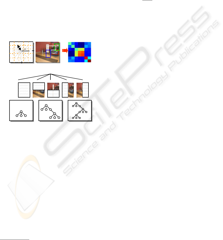
Figure 1: (i) Points sampled to calculate the LBP around a
point (x,y). (ii) Rectangles are examples of possible regions
for histogram features. Stable appearance in Rectangles A,
B and C are good candidates for a car classifier while re-
gions D is not. (iii) Any region can be represented by a
covariance matrix. Size of the covariance matrix is propor-
tional to the number of features used. Second row shows an
object represented with five covariance matrices. The third
row shows an example of forest structure for a given ob-
ject. In our example, it can be seen that the tree adapts the
decision at each intermediate node (nonterminal) from the
response of the leaf nodes, which characterized by a vector
(w
i
,C
i
) with
k
w
i
k
= 1.
2.1 Our Approach
To overcome the above mentioned shortcomings in
object descriptors, we have used bag of covariance
2
matrices, to represent an object region.
Let I be an input color image. Let F be the dimen-
2
Basically, covariance is a measure of how much two
variables vary together.
sional feature image extracted from I
F(x,y) = φ(I,x,y) (1)
where the function φ can be any feature maps (such
as intensity, color, etc). For a given region R ⊂ F, let

f
j

j=1···n
be the d dimensional feature points inside
R. We represent the region R with the d × d covari-
ance matrix C
R
of feature points.
C
R
=
1
n − 1
n
∑
j=1
( f
j
− µ)( f
j
− µ)
T
(2)
where µ is the mean of the point. Fig.1 (i) depicts the
points that must be sampled around a particular point
(x,y) in order to calculate the LBP at (x,y). In our im-
plementation, each sample point lies at a distance of 2
pixels from (x,y), instead of the traditional 3 × 3 rect-
angular neighborhood, we sample neighborhood cir-
cularly with two different radii (1 and 3). The result-
ing operators are denoted by LBP
8,1
and LBP
8,1+8,3
,
where subscripts tell the number of samples and the
neighborhood radii. In Fig.1 (ii), different regions of
an object may have different descriptive power and
hence, difference impact on the learning and recogni-
tion.
2.2 Labeling the Image
We gradually build our knowledge of the image, from
features to covariance matrix to a bag of covariance
matrices. Our first step is to model each covariance
matrix as a set of image features. Next, we group
covariance matrices that are likely to share common
label into a bag of covariance matrices. We follow
(Tuzel, 2006) and represent an image objects with
five covariance matrices C
i=1···5
of the feature com-
puted inside the object region, as shown in the sec-
ond row of Fig.1. A bag of covariance which is nec-
essary a combination of Ohta color space histogram
(I
1
= R + G + B/3, I
2
= R − B, I
3
= (2G − R − B)/2),
LBP and appearance model of different features of an
image window is presented in Fig.1 (iii). Then esti-
mate the bag of covariance matrix likelihoods and the
likelihood that each bag of covariance matrices is ho-
mogeneously labeled. We use this representation to
automatically detect any target in images. We then
apply on-line RF learner to select object descriptors
and to learn an object classifier, as cab be seen in the
last row of Fig.1.
2.3 Incremental Feature Selection
Our incremental feature selection implementation
performs the same sort of incremental hill-climbing
search for generating a concept hierarchy known as
IMAGAPP 2009 - International Conference on Imaging Theory and Applications
6

sequential selection. We resort to an implementation
that uses forward selection (FS). The FS algorithm is
shown in Algorithm.1, start with no variables F
0
= φ
and then during each run m adds a new set f ` of fea-
tures. As can be seen in Eq.(3), the set of all features
at stage m is denoted by F
m
, where F
m
is the union
of features that have just arrived with the set of fea-
tures that was selected at stage m − 1. At each step
and greedily adding the one that enhances the evalu-
ation and decreases the error most, until any further
addition does not significantly decreases the error.
F
m
= F
m−1
∪
{
f`
}
, (3)
where
f` = arg max
F
m−1
∩
{
f `
}
=φ
Q(F
m−1
∪
{
f`
}
) (4)
Algorithm 1: Forward Feature Selection.
1: LET feature f (0) = φ; error(0) = +∞
2: LET feature subset f (0) = all
3: for m = 1,2,··· , the number of all features
in random subset do
4: LET f (m) = f (m − 1)∪ the m-th best feature in
F(0)
5: Perform a training with f (m) to obtain error rate
error(m)
6: end for
7: IF error(m) > error(m − 1) THEN terminate
feature select and
8: RETURN f (m −1)
9: NEXT m
3 RANDOM FORESTS FOR
RECOGNITION
In the following we introduce the on-line random
forests learning algorithm (Elgawi, 2008) for object
recognition based on Breiman’s random forest (RF)
(Breiman, 2001). Details discussion of Breiman’s
random forest learning algorithm is beyond the scope
of this paper, however, in order to simplify the further
discussion, we will need to define some fundamental
terms:
Random Forests. (RF) is a tree-based ensemble
prediction technique combining properties of an effi-
cient classifier and feature selection (Breiman, 2001).
Briefly, it is an ensemble of two sources of random-
ness to generate base decision trees; bootstrap repli-
cation of instances for each tree and sampling a ran-
dom subset of features at each node. It is also enable
different cues (such as appearance and shape) to be
combined (Winn, 2006). RFs classifiers have been
applied to object recognition (Moomsmann, 2006;
Winn, 2006) but only for a relatively small number
of classes.
Feature Importance Estimation. RF measures
feature importance by randomly permuting the values
of the feature f for the out-of-bag (OOB)
3
cases for
tree k, if feature f is important in the object detection,
then the accuracy of the prediction should decrease.
On the other hand, we can consider the accumulated
reduction at nodes according to the criteria used at
the splits, an idea from the original CART (Breiman,
1984) formulation. Feature importance measures can
be used to perform object descriptors selection.
Decision Tree. For the k-th tree, a random covari-
ance matrix C
k
is generated, independent of the past
random covariance matrices C
1
,.. .,C
k
−1
, and a tree is
grown using the training set of positive and negative
image I and covariance feature C
k
. The decision gen-
erated by a decision tree corresponds to a covariance
feature selected by learning algorithm. Each tree casts
a unit vote for a single matrix from the bag of covari-
ance matrices.
Base Classifier. Given a set of M decision trees, a
base classifier selects exactly one decision tree classi-
fier from this set, resulting in a classifier h(I,C
k
).
Forest. Given a set of N base classifiers, a forest
is computed as ensemble of these tree-generated base
classifiers h (I,C
k
), k = 1,.. .,n. Finally, a forest de-
tector is computed as a majority vote.
Majority Vote. If there are M decision trees, the
majority voting method will give a correct decision
if at least f loor(M/2) +1 decision trees gives correct
outputs. If each tree has probability p to make a cor-
rect decision, then the forest will have the following
probability P to make a correction decision.
P =
b
∑
i=floor(M/2)+1

M
i

p(1 − p) (5)
3.1 On-line Learning Random Forest
To obtain an on-line algorithm, each of the steps
described above must be on-line, where the current
3
There is on average I/e ≈ 36.8 of instances not tak-
ing part in construction of the tree, provides a good esti-
mate of the generalization error (without having to do cross-
validation).
INCREMENTAL MACHINE LEARNING APPROACH FOR COMPONENT-BASED RECOGNITION
7

Algorithm 2: On-line Random Forests.
1: Input: training set T , integer N
(No. of bootstrap)
2: Use all available sample so far d to learn feature
descriptors.
3: Estimate the importance of feature incrementally.
4: Restrict d to the relevant features.
5: Train RF based on the restricted data d as
follows.
——————————————-
6: Initially select the number K of trees to be
generated.
7: for k = 1, 2, · · · ,K do
8:
`
T
¯
bootstrap sample from T initialize
e = 0,t = 0, T
k
= φ
9: Do until T
k
= N
k
10: Vector C
k
that represent a bag of covariance is
generate
11: Construct Tree h (I,C
k
) using any decision tree
algorithm
12: Each Tree makes its estimation based on a
single matrix from the bag of covariance
matrices at I.
13: Each Tree casts a vote for most popular
covariance matrix at I
14: The popular covariance matrix at I at is
predicted by selecting the matrix with
max votes over h
1
,h
2
,...,h
k
15: = arg max
y
∑
K
k=1
I(h
k
(x) = y)
16: Return a hypothesis h
l
17: end for
18: Get the next sample set (x, y) in
`
Tt ← t + 1 t
(is the number of sample sets examined in the
process)
19: Output: Proximity measure, feature importance
, a hypothesis h.
classifier is updated whenever a new sample arrives.
In particular on-line RF (Elgawi, 2008) (see Algo-
rithm.2) works as follows: First, based on covari-
ance object descriptor we develop a new, conditional
permutation scheme for the computation of variable
importance measure. The resulting incremental vari-
able importance is show to reflect the true impact of
each predictor variable more reliably than the original
marginal approach. Second, the fixed set tree K is ini-
tialized. In contrast to off-line random forests, where
the root node always represents the object class in on-
line mode, for each training sample, the tree adapts
the decision at each intermediate node (nonterminal)
from the response of the leaf nodes, which character-
ized by a vector (w
i
,C
i
) with
k
w
i
k
= 1. Root node
numbered as 1, the activation of two child nodes 2i
and 2i + 1 of node i is given as
u
2i
= u
i
. f (w
0
i
I +C
i
) (6)
u
2i+1
= u
i
. f (−w
0
i
I +C
i
) (7)
input
Positive training images
Negative training images
Offline Training
Base
Compute covariance
and train classifiers
Base
Base
Base
accept
reject
reject
reject
reject
Random Forests Classifier
D Tree D TreeD Tree
Scan Image Windows
Base
No Human
Base
No Human
Base
No Human
Base
No Human
Human
Detected Human
Online Detection
),(
11
θω
),(
44
θ
ω
),(
33
θ
ω
),(
55
θ
ω
),(
22
θ
ω
)1)1((
=
u
Random Forests Classifier
D Tree D TreeD Tree
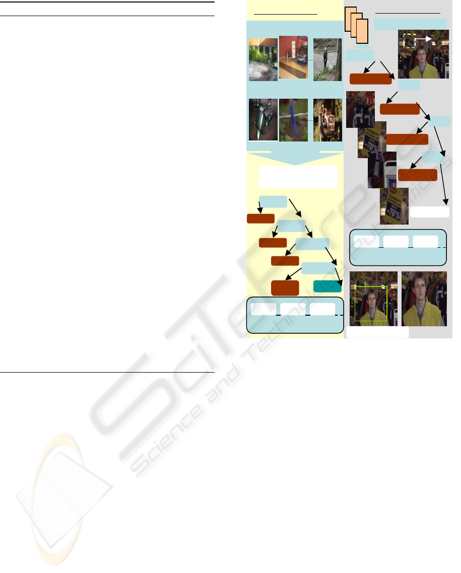
Figure 2: A classifier is trained with positive (contains the
object relevant to the class) and negative (does not contain
the object) examples. Each decision tree makes its estima-
tion based on a single matrix from the bag of covariance
matrices.
where I is the input image, u
i
represents the activation
of node i, and f (.) is chosen as a sigmoidal function.
Consider a sigmoidal activation function f (.), the sum
of the activation of all leaf nodes is always unity pro-
vided that the root node has unit activation. The for-
est consist of fully grown trees of a certain depth l.
The general performance of the on-line forests de-
pends on the depth of the tree. However, we found
that the number of trees one needs for good perfor-
mance eventually tails off as new data vectors are con-
sidered. Since after a certain depth, the performance
of on-line forest does not vary to a great extent, the
user may choose K (the number of trees in forest) to
be some fixed value or may allow it to grow up to the
maximum possible which is at most
|
T
|
/N
k
, where N
k
the tree size chosen by the user.
IMAGAPP 2009 - International Conference on Imaging Theory and Applications
8

4 OBJECT RECOGNITION
Given a feature set and a sample set of positive (con-
tains the object relevant to the class) and negative
(does not contain the object) images, to detect a spe-
cific object, e.g. human, in a given image, the main
difficulty is to train a classifier with relevant features
toward accurate object recognition. The adoption of
RF learner and its ability to measure feature impor-
tance relief us from this challenge. We train a random
forests learner (detector) offline using covariance de-
scriptors of positive and negative samples as shown
in Fig. 2 (left column). We start by evaluation fea-
ture from input image I after the detector is scanned
over it at multiple locations and scales. This has to
be done for each object. Then for feature in I, we
want to find corresponding covariance matrix for es-
timating a decision tree. Each decision tree learner
may explore any feature f , we keep continuously ac-
cepting or rejecting potential covariance matrices. We
then apply the on-line random forests at each candi-
date image window to determine whether the window
depicts the target object or not as shown in Fig. 2
(right column). The on-line RF detector was defined
as a 2 stage problem, with 2 possible outputs in each
stage: In the first one, we build a detector that can
decide if the image contains an object, and thus must
be recognized, or if the image does not contain ob-
jects, and can be discarded, saving processing time.
In the second stage, based on selected features the de-
tector must decide which object descriptor should be
used. There are two parameters controlling the learn-
ing recognition process: The depth of the tree, and
the least node. It is not clear how to select the depth
of the on-line forests. One alternative is to create a
growing on-line forests where we first start with an
on-line forest of depth one. Once it converges to a lo-
cal optimum, we increase the depth. Thus, we create
our on-line forest by iteratively increasing its depth.
4.1 Detection Instances
Next, when detecting a new instance, we first estimate
the average margin of the trees on the instances most
similar to the new instance and then, after discarding
the trees with negative margin, weight the tree’s votes
with the margin. Then the set of classifiers is updated.
For updating, any on-line learning algorithm may be
used, but we employ a standard Karman filtering tech-
nique (karman, 1990) and build our adaptive model
by estimate the probability P(1| f
j
x) with mean µ
+
and standard deviation σ
+
for positive samples and
P(−1| f
j
(x)) by N(µ
−
,σ
−
) for negative samples sim-
ilar way as we do in the off-line case.
Table 1: Number of images and objects in each class in the
GRAZ02 dataset.
Dataset Images Objects
Bikes 373 511
Cars 420 770
Persons 460 785
Total 1253 2066
5 EXPERIMENTS AND
EVALUATION
To evaluate and validate our approach, we designed
our experiments in a way that we can answer the fol-
lowing questions:
1. How does the performance of incrementally learn-
ing RF compare to one trained batch on the entire
training set?
2. Does the recognition performance improve it uses
covariance matrices rather than adapting His-
tograms?
5.1 Dataset
To investigate the above questions we used data de-
rived from the GRAZ02
4
dataset (Oplet, 2006), a col-
lection of 640 × 480 24-bit color images. As Fig.3
illustrates, the GRAZ02 database contains variability
with respect to scale and clutter. Objects of interest
are often occluded, and they are not dominant in the
image. According to (Oplet, 2005) the average ratio
of object size to image size counted in number of pix-
els is 0.22 for bikes, 0.17 for people, and 0.9 for cars.
Thus this dataset is more complex dataset to learn de-
tectors from, but of more interest because it better re-
flects the real world complexity. As can be seen in Ta-
ble 1, this dataset has three object classes, bikes (373
images), cars (420 images) and persons (460 images),
and a background class (270 images).
5.2 Experimental Settings
For testing our framework we used the datasets de-
scribed above and run it against three state of the art
classifiers (offline RF, AdaBoost, and SVM). Each
of the classifiers used in our experimentation were
trained with varying amounts (10%,50% and 90% re-
spectively) of randomly selected training data. All
image not selected for the training split were put into
the test split. For the 10% training data experiments,
4
available at htt://www.emt.tugraz.at/pinz/data/
INCREMENTAL MACHINE LEARNING APPROACH FOR COMPONENT-BASED RECOGNITION
9

10% of the image were selected randomly with the re-
mainder used for testing. This was repeated 20 times.
For the 50% training data experiments, stratified 5x2
fold cross validation was used. Each cross validation
selected 50% of the dataset for training and tested the
classifiers on the remaining 50%; the test and training
sets were then exchanged and the classifiers retrained
and retested. This process was repeated 5 times. Fi-
nally, for the 90% training data situation, stratified
1x10 fold cross validation was performed, with the
dataset divided into ten randomly selected, equally
sized subsets, with each subset being used in turn for
testing after the classifiers were trained on the remain-
ing nine subsets. For offline random forests, we train
detectors for bikes, cars and persons on 100 positive
and 100 negative images (of which 50 are drawn from
the other object class and 50 from the background),
and test on a similarly distributed set.
6 EXPERIMENTAL RESULTS
GRAZ02 images contain only one object category per
image so the recognition task can be seen as a bi-
nary classification problem: bikes vs. background,
people vs. background, and cars vs. background.
The well known statistic measure; the Area Under the
ROC Curve (AUC) is used to measure the classifiers
performance in these object recognition experiments.
The AUC is a measure of classifier performance that
is independent of the threshold: it summarizes not the
accuracy, but how the true positive and false positive
rate change as the threshold gradually increases from
0.0 to 1.0. An ideal, perfect, classifier has an AUC
value 1.0 while a random classifier has an AUC of
0.5.
6.1 Mean AUC Performance
Tables 2, 3, and 4 give the mean AUC values across
all runs to 2 decimal places for each of the classifier
and training data amount combinations, for the bikes,
cars ad people datasets respectively. For on-line RF
we report the results for different depths of the tree.
As can be seen, our algorithm always performs sig-
nificantly better than the offline RF. We found that the
differences in performance are (avg. = 1.2 ± 15%),
while our approach has achieved a number of desir-
able properties: (1) it is incremental, in a sense that
we are able to add new categories incrementally mak-
ing use of already acquired knowledge, the model will
continuously improve by exploring more features and
training data. If the process is running for a long time,
a lot of features are processed and evaluated but still
only a small number of features are sufficient for up-
dating. (2) it is adaptable, in a sense that the selection
of features and also the learning (we do not freeze the
learning) can change over time. Note that this kind
of adaptively is not possible in the standard random
forests and the other batch learning classifiers. Such
capability of on-line adaptation would take us closer
to the goal of more versatile, robust and adaptable
recognition system. The improvement when we vary-
ing the tree depth are relatively small. This makes
intuitive sense: when an image is characterized by
high geometric variability, it is difficult to find useful
global features.
6.2 A Bag of Covariance vs. Histograms
Another objective of the experiments was to de-
termine whether a bag of covariance matrices can
improve the recognition performance of histogram
methods. Covariance features are faster than the
histogram since the dimensionality of the space is
smaller. The search time of an object in 24-bit color
image with size 640 × 480 is 8.5 (s) with C++ im-
plementation which yield near real time performance.
The main computational effort is spend for updating
the base classifiers. In order to decrease computation
time we use a method similar to (Wu, 2003). Assum-
ing all feature pools are the same F
1
= F
2
= ··· = F
M
,
then we can update all corresponding base classi-
fiers only once. This speeds up the process consider-
ably while only slightly decreasing the performance.
We noted that the standard deviation varies between
±2.0 ± 3.2, which is considered quite high. The rea-
son is the images in the dataset vary greatly in their
level of difficulty, so the performance for any single
run is dependent on the composition of the training
set.
6.3 On-line Recognition Learning vs.
Offline Learning
Without loss of generality, the method we propose
is able to learn completely in the on-line mode, and
since we do not freeze the learning, it can adapt to a
changing situation. There are two reasons why this
choice of incremental learning of object recognition
may be useful. First of all, a machine has a com-
petitive advantage if it can immediately use all the
training data collected so far, rather than wait for a
complete training set. Second, search efficiency can
significantly improve due to the use of covariance de-
scriptor, which is consider more closet represent the
object choice shape.
IMAGAPP 2009 - International Conference on Imaging Theory and Applications
10

Figure 3: Examples from GRAZ02 dataset (Oplet, 2006) for four different categories: bikes (1st pair), people (2nd pair), cars
(3rd pair), and background (4th pair).
Table 2: Mean AUC performance of four classifiers on the Bikes vs. Background dataset, by amount of training data.
Performance of on-line RF is reported for different Depths.
On-line RF with different depth (Dth) Offline AdaB SVM
Dth=3 Dth=4 Dth=5 Dth=6 Dth=7 RF
10% 0.85 0.86 0.81 0.85 0. 85 0.86 0.81 0.82
50% 0.91 0.90 0.89 0.91 0.92 0.90 0.89 0.90
90% 0.92 0.90 0.91 0.92 0. 92 0.91 0.90 0.91
Table 3: Mean AUC performance of four classifiers on the Cars vs. Background dataset, by amount of training data. Perfor-
mance of on-line RF is reported for different Depths.
On-line RF with different depth (Dth) Offline AdaB SVM
Dth=3 Dth=4 Dth=5 Dth=6 Dth=7 RF
10% 0.77 0.79 0.75 0.78 0.73 0.79 0.75 0.73
50% 0.85 0.84 0.82 0.82 0.84 0.85 0.82 0.80
90% 0.86 0.82 0.83 0.85 0.86 0.85 0.83 0.82
Table 4: Mean AUC performance of four classifiers on the Persons vs. Background dataset, by amount of training data.
Performance of on-line RF is reported for different Depths.
On-line RF with different depth (Dth) Offline AdaB SVM
Dth=3 Dth=4 Dth=5 Dth=6 Dth=7 RF
10% 0.84 0.84 0.83 0.80 0.83 0.84 0.77 0.80
50% 0.88 0.86 0.88 0.88 0.88 0.88 0.84 0.86
90% 0.90 0.86 0.89 0.90 0.90 0.90 0.86 0.89
7 CONCLUSIONS
In this paper we have presented an on-line learn-
ing framework for object recognition categories that
avoids hand labeling of training data. We have
demonstrated that on-line learning obtain compara-
ble results to offline learning. Moreover, the proposed
framework is quite general (i.e, it can be used to learn
completely different objects) and can be extended in
several ways. Although we assess the problem of pro-
ducing accurate object recognition in images, without
giving any prior information on object identities, ori-
entation, positions and scales, but we still far behind
than proposing a multi-general vision task algorithm
but our hope is to design a simple algorithm for learn-
ing appropriate context for object recognition tasks in
similar hierarchical and parallel processing of human
brain.
REFERENCES
O. Tuzel, F. Porikli, and P. Meer. “Region covariance: A fast
descriptor for detection and classification,” In Proc.
ECCV, 2006.
A, Opelt., & A, Pinz. (2005). Object Localization with
boosting and weak supervision for generic object
recognition. In Kalvianen H.‘et al.’. (Eds.). In Proc.
SCIA 2005, LNCS 3450, pp. 862-871.
B, Schiele., & J, L. Crowley. (2000). Recognition with-
out correspondence using multidimensional receptive
field histograms. IJCV. 36(1):3150
D, G. Lowe. (1999). Object recognition from local scale-
invariant features. In Proc. ICCV. pp. 11501157.
F, Moomsmann., B, Triggs., & F, Jurie. (2006). Fast dis-
criminative visual codebooks using randomized clus-
tering forests. NIPS.
H, Schneiderman & T, Kanade. (2000). A statistical method
INCREMENTAL MACHINE LEARNING APPROACH FOR COMPONENT-BASED RECOGNITION
11

for 3D object detection applied to faces and cars. In
Proc. CVPR. volume I, pp. 746751
Hassab Elgawi Osman. (2008). Online Random Forests
based on CorrFS and CorrBE. In Proc.IEEE workshop
on online classification, CVPR. pp. 1–7
J, Wu., J, Rehg., & M, Mullin. (2003). Learning a rare event
detection cascade by direct feature selection. In Proc.
NIPS.
J, Winn., & A, Criminisi. (2006). Object class recognition
at a glance. CVPR.
K. P, Karman., & A. von Brandt. (1990). Moving object
recognition using an adaptive background memory in
Time-varying Image Processing and Moving Object
Recognition. Capellini, Ed.. volume. II. Amsterdam,
The Netherlands: Elsevier, pp. 297307.
L, Breiman. (2001). Random Forests. Machine Learning.
45(1):5.32.
L, Breiman, Jerome H. Friedman, Richard A. Olshen, &
Charles J. Stone. (1984). Classification and regression
trees. Wadsworth Inc.. Belmont, California.
M, J. Swain., & D, H. Ballard. (1999). Color indexing.
IJCV. 7(1):1132
Oplet A., Fussenegger M., Pinz A., & Auer P. (2006).
Generic object recognition with boosting. IEEE
Transactions on Pattern Analysis and Machine Intel-
ligence. 28(3) pp. 416–431.
O, Tuzel., F, Porikli., & P, Meer. (2006). Region covariance:
A fast descriptor for detection and classification. In
Proc. ECCV.
S. Belongie., J. Malik., & J. Puzicha. (2004). Shape
matching and object recognition using shape contexts.
IEEE-PAMI. 24(4):509522
T. Leung., & J. Malik. (2000). Representing and recogniz-
ing the visual appearance of materials using three-
dimensional textons. IJCV. 43(1):29-44
IMAGAPP 2009 - International Conference on Imaging Theory and Applications
12