ROBUSTNESS OF DIFFERENT FEATURES FOR ONE-CLASS

CLASSIFICATION AND ANOMALY DETECTION IN WIRE ROPES

Esther-Sabrina Platzer, Joachim Denzler, Herbert S¨uße

Chair for Computer Vision, Friedrich Schiller University of Jena, Ernst-Abbe-Platz 2, 07743 Jena, Germany

Josef N¨agele, Karl-Heinz Wehking

Insitute for Mechanical Handling and Logistics, University of Stuttgart, Holzgartenstrae 15B, 70174 Stuttgart, Germany

Keywords:

Anomaly detection, Novelty detection, One-class classiﬁcation, Linear prediction, Local binary pattern.

Abstract:

Automatic visual inspection of wire ropes is an important but challenging task. Anomalies in wire ropes

usually are unobtrusive and their detection is a difﬁcult job. Certainly, a reliable anomaly detection is essential

to assure the safety of the ropes. A one-class classiﬁcation approach for the automatic detection of anomalies

in wire ropes is presented. Different well-established features from the ﬁeld of textural defect detection are

compared to context-sensitive features extracted by linear prediction. They are used to learn a Gaussian

mixture model which represents the faultless rope structure. Outliers are regarded as anomaly. To evaluate

the robustness of the method, a training set containing intentionally added, defective samples is used. The

generalization ability of the learned model, which is important for practical life, is exploited by testing the

model on different data sets from identically constructed ropes. All experiments were performed on real-life

rope data. The results prove a high generalization ability, as well as a good robustness to outliers in the training

set. The presented approach can exclude up to 90 percent of the rope as faultless without missing one single

defect.

1 INTRODUCTION

Wire ropes are used in many ﬁelds of logistics. They

are deployed as load cable for bridges, elevators and

ropeways. This implies a high strain by external pow-

ers every day. Unfortunately, this can lead to struc-

tural anomalies or even defects in the rope formation.

A defectiverope bears a high risk for human life. This

motivates the strict rules summarized in the European

norm (EN 12927-7, 2004), which instruct a regular

inspection of wire ropes .

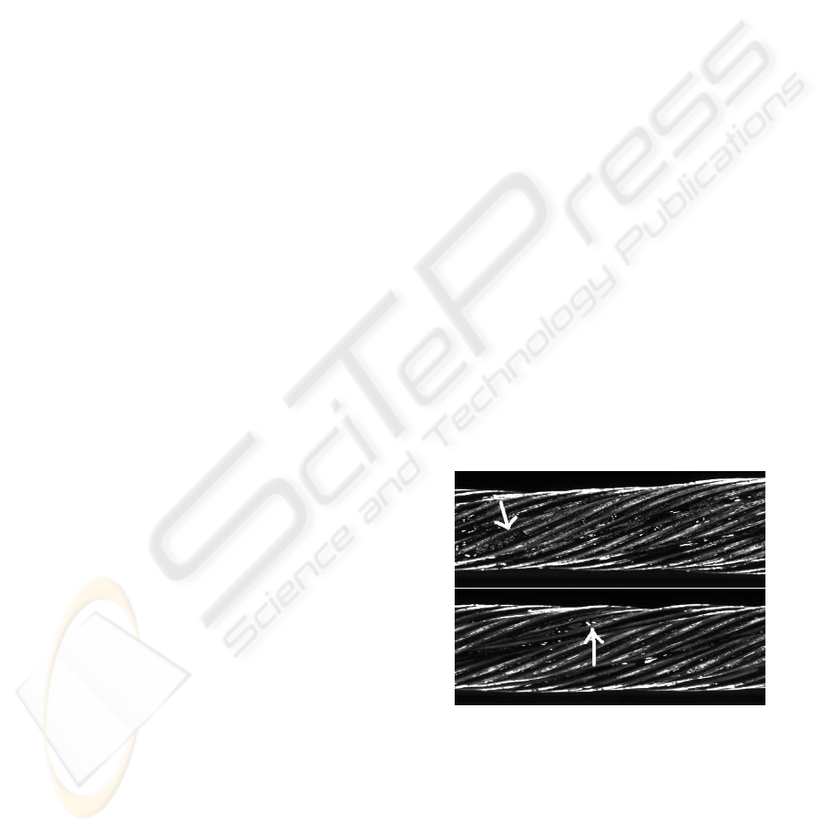
Risky defects, prominent in wire ropes, are small

wire fractions, missing wires, and damaged rope ma-

terial due to lightening strokes. Furthermore, struc-

tural anomalies caused by interweavement of the rope

ends or a reduced stress are also in the focus of in-

terest. In ﬁgure 1, two exemplary defects are marked

in the rope. Visual inspection of wire ropes is a difﬁ-

cult and dangerous task. Besides, the inspection speed

is quite high (on average 0.5 meters/second) which

makes it a hard effort, to concentrate on the passing

rope without missing small defective rope regions.

Figure 1: Rope defects: in the upper image you can see a

wire fraction and in the image below a wire is missing.

A prototypic acquisition system was developed to

overcome these limitations (Moll, 2003). Four line

cameras record the passing rope and yield four differ-

ent views. By this, the rope can be inspected in the

ofﬁce without time pressure. The images in ﬁgure 1

were acquired with this system.

Defects and anomalies in wire ropes are unimposing

171

Platzer E., Denzler J., Süße H., Nägele J. and Wehking K. (2009).

ROBUSTNESS OF DIFFERENT FEATURES FOR ONE-CLASS CLASSIFICATION AND ANOMALY DETECTION IN WIRE ROPES.

In Proceedings of the Fourth International Conference on Computer Vision Theory and Applications, pages 170-177

DOI: 10.5220/0001783801700177

 SciTePress

and small. The image quality is deranged by mud,

powder, grease or water and the lighting conditions

change frequently. Therefore, the choice of features

for the detection task is important. Recent approaches

for defect or anomaly detection focus on fault de-

tection in material-surfaces. In (Platzer et al., 2008)

we introduced a one-class classiﬁcation approach for

anomaly detection in wire ropes using linear predic-

tion (LP) coefﬁcients as features and a Gaussian mix-

ture for model learning. The former work is ex-

tended in this paper by two main aspects: the per-

formance of LP features is compared to that of other

well-established features from the ﬁeld of textural de-

fect detection, and the robustness to outliers in the

training set as well as the generalization ability of

the presented approach are carefully evaluated. The

last point is of particular interest for the practical rel-

evance of the method.

Features based on local binary patterns (LBP)

were ﬁrst introduced by Ojala (Ojala et al., 1996)

for texture classiﬁcation. Recently they were used

for defect detection in fabrics (Tajeripour et al.,

2008) and for real-time surface inspection (M¨aenp¨a¨a

et al., 2003). Textural features, extracted from co-

occurrence matrices, were proposed by Harlick in

the early 70’s (Harlick et al., 1973) and are fre-

quently used for texture description (Chen et al.,

1998). (Iivarinen, 2000) compares two histogram-

based methods for surface defect detection using LBP

and co-occurrence matrices. (Rautkorpi and Iivari-

nen, 2005) used shaped-based co-occurrence matrices

for the classiﬁcation of metal surface defects. (Vartia-

ninen et al., 2008) focus on the detection of irregular-

ities in regular, periodic patterns. They separate the

image data in a regular and an irregular part. Based

on the resulting irregularities, we compute local his-

tograms, which serve as features. Another important

category of features for texture analysis and textural

defect detection are wavelet-based features. (Kumar

and Pang, 2002) for example use Gabor features for

the detection of defects in textured material. How-

ever, the computation of these features requires large

ﬁlter banks and high computational costs. Due to

the huge size of rope data sets (20-30 GB) the time-

consuming computation of Gabor features seems to

be not the best choice. In (Varma and Zisserman,

2003) the authors state, that similar results to that

obtained by the usage of wavelet features can be re-

solved with help of joint neighborhood distributions

and less computational effort.

The one-class classiﬁcation strategy proposed in

(Platzer et al., 2008) was chosen due to a lack of de-

fective training samples for supervised classiﬁcation.

In contrast, it is no problem to design a huge sample

set of faultless training samples. With this faultfree

training set a model of the intact rope structure can

be learned and in the detection step outliers with re-

gard to this model are classiﬁed as defect. However,

the only available ground truth information about this

training data is the labeling of the human expert. In

the following,there remains a small uncertainty of un-

derdiagnosed defects in the training set. For this rea-

son the robustness of the proposed method to outliers

in the training set is evaluated. Results obtained by

learning from a faultless training set are compared to

those, obtained by learning from a training set with

intentionally added, faulty samples. The generaliza-

tion ability of a learned model is a further important

point, especially for the practical relevance of the pre-

sented method. There exist only a limited number of

different construction types for wire ropes. The dif-

ferences between them are mainly a different num-

ber of wires and strands, different thickness of single

wires, the length of twist and the diameter. If just one

model for every possible rope type would have to be

learned in advance, this would save a lot of compu-

tational effort. However, the rope data from different

ropes differs signiﬁcantly due to the changing acquisi-

tion conditions and a different mounting of the ropes.

Nevertheless, it is desirable to have just one model

for every construction type and to overcome the chal-

lenges of a changing acquisition environment. There-

fore, the generalization ability of the learned models

is evaluated by learning and testing on different rope

data from nearly identical constructed ropes.

The paper is structured as follows: in section 2 we

brieﬂy review the feature extraction using linear pre-

diction and give a description of the used textural fea-

tures and their extraction. The one-class classiﬁcation

of wire rope data is shortly summarized in section 3.

Experiments, revealingthe usability and robustness of

our approach, have been performed on real-life rope

data and results are presented in section 4. A conclu-

sion and a discussion about future work is given in

section 5.

2 FEATURE EXTRACTION

In this section the different features are brieﬂy re-

viewed. Their extraction from the underlying rope

data is described, as it differs for the LP features in

contrast to the remaining features. In the following, a

short motivation for the different features used in this

context, is given.

Local binary patterns (LBP) code the local

graylevel-structure of a pixel neighborhood. His-

tograms based on the resulting codes lead to a local

VISAPP 2009 - International Conference on Computer Vision Theory and Applications

172

feature distribution. Since local binary patterns incor-

porate contextual information from a local neighbor-

hood, a comparison of their performance with that of

the LP features is of particular interest.

(Harlick et al., 1973) introduced a set of 14 dif-

ferent textural features computed from co-occurrence

matrices. They reveal the spatial distribution of gray-

levels an though seem to be an interesting choice for

structures with a certain regularity, like wire ropes.

The detection of irregularities, proposed in (Var-

tianinen et al., 2008) focuses on anomalies in regular,

periodic patterns. Since the structure of wire ropes

is not perfectly periodic, but offers some regular pe-

riodicities, we used the detected irregularities for the

computation of local, histogram-based features.

2.1 Linear Prediction Based Features

Linear prediction can be seen as one key technique in

speech recognition (Rabiner and Juang, 1993). It is

used to compute parameters determining the spectral

characteristics of the underlying speech signal.

The behavior of the underlying signal is modelled

by forecasting the value x(t) of the signal x at time t

by a linear combination of the p past values x(t − k)

with k = 1, . . . , p, where p is the order of the autore-

gressive process. The prediction ˆx(t) of a 1-D signal

can be written as

ˆx(t) = −

∑

k=1

x(t − k) (1)

with the following prediction error

e(t) = x(t) − ˆx(t) = x(t) +

∑

k=1

x(t − k). (2)

This motivates the choice of linear prediction for fea-

ture extraction. For the prediction of the actual value

the contextual information of the past values is used

and is implicitly incorporated in the resulting feature.

Based on a least-squares formulation, the opti-

mal parameters

α = (1, α

... α

) can be obtained by

solving the normal equations (Makhoul, 1975). The

optimal coefﬁcients are derived by use of the auto-

correlation method and the Levinson-Durbin recur-

sion (Makhoul, 1975; Rabiner and Juang, 1993). Free

parameters of this method are framesize and the order

of the process. In experiments the optimal framesize

was found to be 20 camera lines with an incremen-

tal overlap of 10 lines. Best results were achieved for

order p = 8.

Rope data, obtained from the acquisition system,

can be seen as a sequence of 2-d images. Thus,

with 1-d linear prediction it is not possible to ana-

lyze the 2-d signal. To overcome this, the rope data

Figure 2: Multichannel version of the classiﬁcation model.

For every channel (horizontal white boxes) a feature is ex-

tracted and examined in a separate feature space. The ver-

tical white box marks the signal values, which are actually

predicted.

is considered as a multichannel time series. The sig-

nal ~x consists of c channels ~x = (~x

...~x

)

and

every channel represents a 1-dimensional time se-

ries ~x

(t) = (x

(1),... , x

(t)). For every channel i of

this signal an individual 1-d linear prediction is per-

formed, leading to the estimate ˆx

(t), the squared pre-

diction error for the whole frame, and the coefﬁcient

vector

. These components are used as correspond-

ing feature for the actual frame and the channel i. Best

results were obtained with a combined feature vector,

including prediction coefﬁcients and the squared er-

ror. In the training step, a separate model for every

channel is learned. This is schematically depicted in

ﬁgure 2. By this, the different appearance of the rope

at different positions in the images is taken into con-

sideration.

2.2 Local Binary Pattern

For the local binary pattern (LBP) a texture region is

seen as a joint distribution of P + 1 pixel-graylevels

in a predeﬁned neighborhood. Often a circular neigh-

borhood with radius R and P equally spaced sam-

ples is chosen. The center pixel grayvalue g

serves

as threshold for the binarization of the neighborhood

pixels g

, p = 1, . . . , P. The local binary pattern oper-

ator can be summarized as follows:

LBP

P,R

) =

∑

p=1

s(g

− g

p−1

(3)

with s(x) =

(

1, x ≥ 0

0, x < 0 .

(4)

Transforming the binary vector into a decimal num-

ber (3) results in a pixel label, based on the neigh-

borhood information. (Ojala et al., 2000) developed a

rotational invariant and uniform extension of the local

binary pattern. For the anomaly detection task there

is no need for rotational invariance due to the constant

rope orientation. The uniformity of the pattern is de-

ﬁned based on the number of 0/1 transitions U in the

binary vector. The resulting LBP code is computed as

ROBUSTNESS OF DIFFERENT FEATURES FOR ONE-CLASS CLASSIFICATION AND ANOMALY DETECTION

IN WIRE ROPES

173

Figure 3: Detection window with 20× 20 pixels in relation

to the wire rope image data.

follows:

LBP

P,R

) =

(

∑

p=1

s(g

− g

), U ≤ 2

P+ 1, otherwise .

(5)

A histogram with a predeﬁned number of bins is built

from the underlying code distribution and serves as

feature. The optimal parameters P and R and the

number of quantization levels for the local histograms

were determined in extensive experiments. We found

the optimal parameter setting to be R = 1, P = 8 with

16 quantization levels for the histogram. As already

mentioned, defects usually have just a small elonga-

tion. Hence, the histogram computation resulting in

the feature vector is done for a small detection win-

dow (20× 20 pixels), which moves over the underly-

ing frame of rope data. To get an impression of the

window size in relation to the rope data, a detection

window is visualized in ﬁgure 3. By this, more than

one feature is obtained for every frame.

2.3 Co-occurrence Features

Features for texture classiﬁcation based on co-

occurrence matrices were ﬁrst introduced by (Harlick

et al., 1973). A co-occurrence matrix is deﬁned with

respect to a certain displacement vector

d = (d

)

and results in the joint distribution of co-occurring

grayvalues. The relative frequency p

, which de-

ﬁnes the co-occurrence of two neighboring grayval-

ues (with respect to

d) i and j, is deﬁned as

(

d) = λ|{(x,y) : I(x, y) = i, I(x+ d

,y+ d

) = j} |

(6)

with i, j ∈ {0. . . G − 1} and G the number of gray lev-

els. I represents an image of size M × N and λ is a

normalization factor such that

∑

(

d) = 1.

Harlick introduced 14 different textural features

(Harlick et al., 1973). Experiments for the determina-

tion of the most discriminative ones were performed.

As the information theoretic texture features named

difference entropy, information measure one, infor-

mation measure two and the maximum correlation

coefﬁcient lead to the best results, a combination of

these four features is used. Furthermore, a displace-

ment vector of 2 pixels length with an angle of 90

degrees has led to the best results in our tests with

varying parameters. As co-occurrence matrices lead

to a global representation of the underlying texture,

they are usually computed for a local region of inter-

est. For the detection of small, regional anomalies in

the rope structure this is important, as the small defect

will not be recognized with global features. Again,

a detection window of 20 × 20 pixels was used for

the computation of the co-occurrencematrices and the

following feature computation.

2.4 Features based on Pattern

Irregularity

(Vartianinen et al., 2008) describe an approach for the

detection of irregularities in regular patterns based on

the Fourier transform. Regular patterns result in dis-

tinct frequency peaks in the Fourier domain. By ﬁl-

tering out these frequencies and transforming the data

back to the spatial domain, a perfectly regular pattern

can be obtained. On the other hand, it is possible to

substract this regular part from a unit function in the

frequency domain, which results in the irregular part

of the pattern:

I(x,y) = F

−1

(I(u,v)) (7)

= F

−1

((1− M(u,v) + M(u, v))I(u,v)) (8)

= F

−1

(M(u,v)I(u,v))

| {z }

regular part

(9)

+ F

−1

((1− M(u,v))I(u,v))

| {z }

irregular part

I(x,y) is the input image, I(u, v) is the Fourier trans-

formed image, F is the Fourier transform and M(u, v)

is the ﬁlter function in the frequency domain. 1 rep-

resents the unit function. Without prior knowledge

about the pattern structure a reasonable ﬁlter func-

tion is self-ﬁltering (Bailey, 1993). Filtering is per-

formed with the magnitude of the Fourier spectrum

M(u,v) = |I(u, v)|. As the rope consists of regular

structures, ﬁltering is done with regard to the irregu-

lar part of the data. For the computation of the local

histograms again a detection window of size 20 × 20

is used. Experimental evaluation of the used quanti-

zation levels for histogram computation showed, that

a histogram with 16 bins performed the best.

3 ONE-CLASS CLASSIFICATION

In order to exclude as many rope meters as possible

from further inspection, the theory of one-class clas-

VISAPP 2009 - International Conference on Computer Vision Theory and Applications

174

siﬁcation seems to be a good choice. A separation be-

tween faultless and faulty samples is required. In this

case, the faultless samples represent the target class

and the defects are considered as outliers ω

. As

it is no problem to construct a large training set of

defect-free feature samples, a representation for this

target density p(~x | ω

) has to be found without any

knowledge about the outlier density p(~x | ω

) (Tax,

2001). Here,~x is the feature vector.

For one-class classiﬁcation problems the false

negative rate (FNR) is the only rate which can be

measured directly from the training data. The false

positive rate (FPR) is the most important measure for

defect detection, but cannot be obtained without a

sample set containing a sufﬁcient number of defective

samples. In case of a uniform distributed outlier den-

sity, however, a minimization of the FNR in combina-

tion with a minimization of the descriptive volume of

the target density p(~x | ω

) results in a minimization

of the FNR and FPR (Tax, 2001).

There exist many different methods for one-class

classiﬁcation (also called novelty detection) (Hodge

and Austin, 2004; Markou and Singh, 2003). In

(Platzer et al., 2008) two approaches, namely the

K-means clustering and a Gaussian mixture model

(GMM), were compared. In contrast to our former

work, where the training sample set contained only

faultless samples, the learning step is now modiﬁed.

Model learning is performed on a sample set with in-

tentionally included samples from defective rope re-

gions. The aim is to evaluate the robustness of the

method against outliers in the training set. This would

reduce the need of a human inspector,who determines

an optimal, faultfree rope region for model learning.

3.1 Decision Making

For a classiﬁcation into target class and outliers, a

threshold is deﬁned on the density. This threshold

is based on the mean and the minimal probability

reached in the training. It is stated, that an optimal

threshold should be within the range of mean and

minimum probability. As the training samples are all

considered as defect-free, the minimum probability

gives the lower bound for the likelihood of faultless

samples. To account for possible outliers, the thresh-

old is varied in this range and the evaluation is done

by means of receiver operating characteristics (ROC).

Since anomaly detection is a security relevant applica-

tion, it is important not to miss any defect. As a con-

sequence, the optimal threshold maximizes the TPR

(number of samples correctly classiﬁed to the target

class) while keeping the FPR zero.

Due to feature extraction with a detection win-

Figure 4: In this rope region a wire is missing. The window

marks the frame, which was detected as an outlier by the

described system.

dow (or in case of the LP features based on one sin-

gle channel), a rope frame consists of more than one

feature. Accordingly, the decision for the overall

frame is based on the decisions for the single win-

dows/channels. In case of feature extraction by a de-

tection window, the frame is classiﬁed as outlier, if

one of the corresponding windows is rejected as out-

lier. For the channel-based LP features a further pre-

processing is necessary. As the channels have no spa-

tial extension like the detection window, one single

channel is prone to noise. Therefore, a local channel-

neighborhoodconsisting of 15 channels is scanned for

potential outliers and only if the number of channel-

votes exceeds ﬁve channels, the whole frame is re-

jected as defect.

Since a defect usually lasts over several frames,

the whole defect is regarded as detected, if one frame

in this range is rejected as outlier. Consequently, de-

fects are detected but not localized at the moment.

Figure 4 displays one defect, detected by the de-

scribed system. The borders of the frame, detected

as outlier are depicted by the window.

4 EXPERIMENTS AND RESULTS

In the following section experiments and their out-

comes are presented. All experiments were per-

formed on authentic rope data, acquired from real

ropeways. In the generalization experiment (subsec-

tion 4.3) the data used for model learning was ac-

quired in a controlled environment, but testing was

again performed on data from a real ropeway. Model

learning was done with a Gaussian mixture composed

of ﬁve mixture components and rope data belonging

to one of the four views. Testing was performed on

all four views and the resulting ROC curves were av-

eraged over the different views. Interference between

the views was not yet considered. The length of the

used rope regions in all experiments is given by the

number of camera lines, followed by the correspond-

ing length in meters put into brackets. Learning on

20.000 camera lines (2m rope) of one view takes be-

tween 25 seconds and one minute on a Intel Pentium

ROBUSTNESS OF DIFFERENT FEATURES FOR ONE-CLASS CLASSIFICATION AND ANOMALY DETECTION

IN WIRE ROPES

175

4 with 3,4GHz, according to the choice of features.

Surely, the LP model learning needs the most time

due to the separate computation of one model for ev-

ery channel. A testrun on 600.000 (60m rope) lines

takes approximately between 14 (Irregularity) and 25

minutes (LP) per view, which gives an average de-

tection speed of 14 till 23 seconds per meter of rope

(10.000 camera lines). Again the computation time

depends on the choice of features.

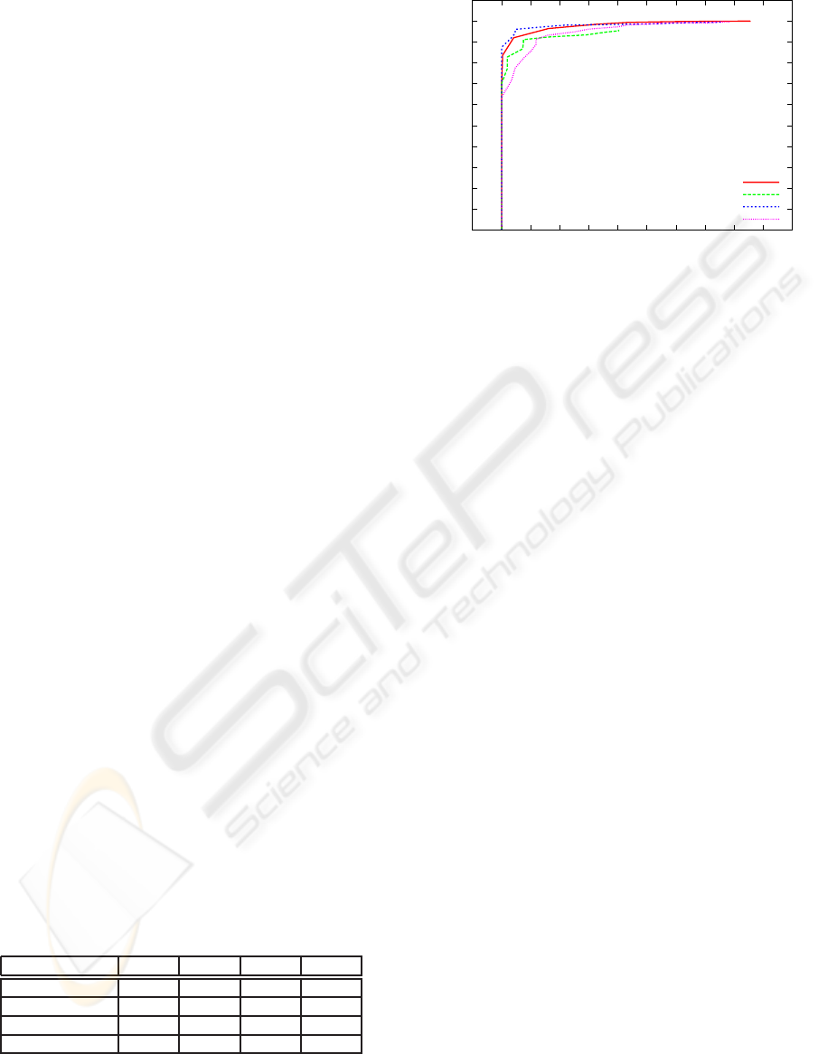
4.1 Comparison of Features

To compare the performance of the different features,

model learning was done for every feature on the

same training set, consisting of 20.000 lines (2m rope)

of defect-free rope data from a real ropeway. Experi-

ments were performed on a connected region of rope

data, containing 600.000 camera lines (60m rope) and

covering all known defects in the rope. The receiver

operating characteristics in ﬁgure 5 point out, that the

LBP features outperform all other features. However,

for all used features respectable results were obtained.

Features based on detected irregularities perform the

worst. A lot of noise is contained in the rope raw

data and the structure is not perfectly regular, so that

a certain amount of irregularities are detected in every

frame. This results in a less discriminative behavior.

Context-sensitive features like the LP features and the

LBP features perform the best. Their overall charac-

teristics show a more robust behavior. Table 1 sum-

marizes the maximum TPR for every view and fea-

ture, which was reached for a FPR of zero. The rea-

son for the decreased TPR of the LP features in view 4

is an easily missed defect in this single view. The un-

derdiagnosed error was manually inspected and it was

discovered, that this defect is spread over more than

one view. In the remaining views this defect was dis-

covered correctly. From this it can be educed, that in-

terference between the different views could be a pos-

sibility to eliminate this misclassiﬁcations. In sum-

mary, these results reveal the importance of context-

sensitive features for the challenging task of defect

detection in wire ropes.

Table 1: Comparison of the maximum TPR for a FPR of

zero for all features and all views.

Featuretype view1 view2 view3 view4

LP 0.96 0.93 0.94 0.62

Co-occurrence 0.78 0.77 0.77 0.88

LBP 0.96 0.82 0.88 0.93

Irregularity 0.62 0.89 0.71 0.78

0.1

0.2

0.3

0.4

0.5

0.6

0.7

0.8

0.9

0 0.1 0.2 0.3 0.4 0.5 0.6 0.7 0.8 0.9 1

True Positive Rate

False Positive Rate

Co-occurrence

LBP

Irregularity

Figure 5: Comparison of the ROC curves for the different

choice of features.

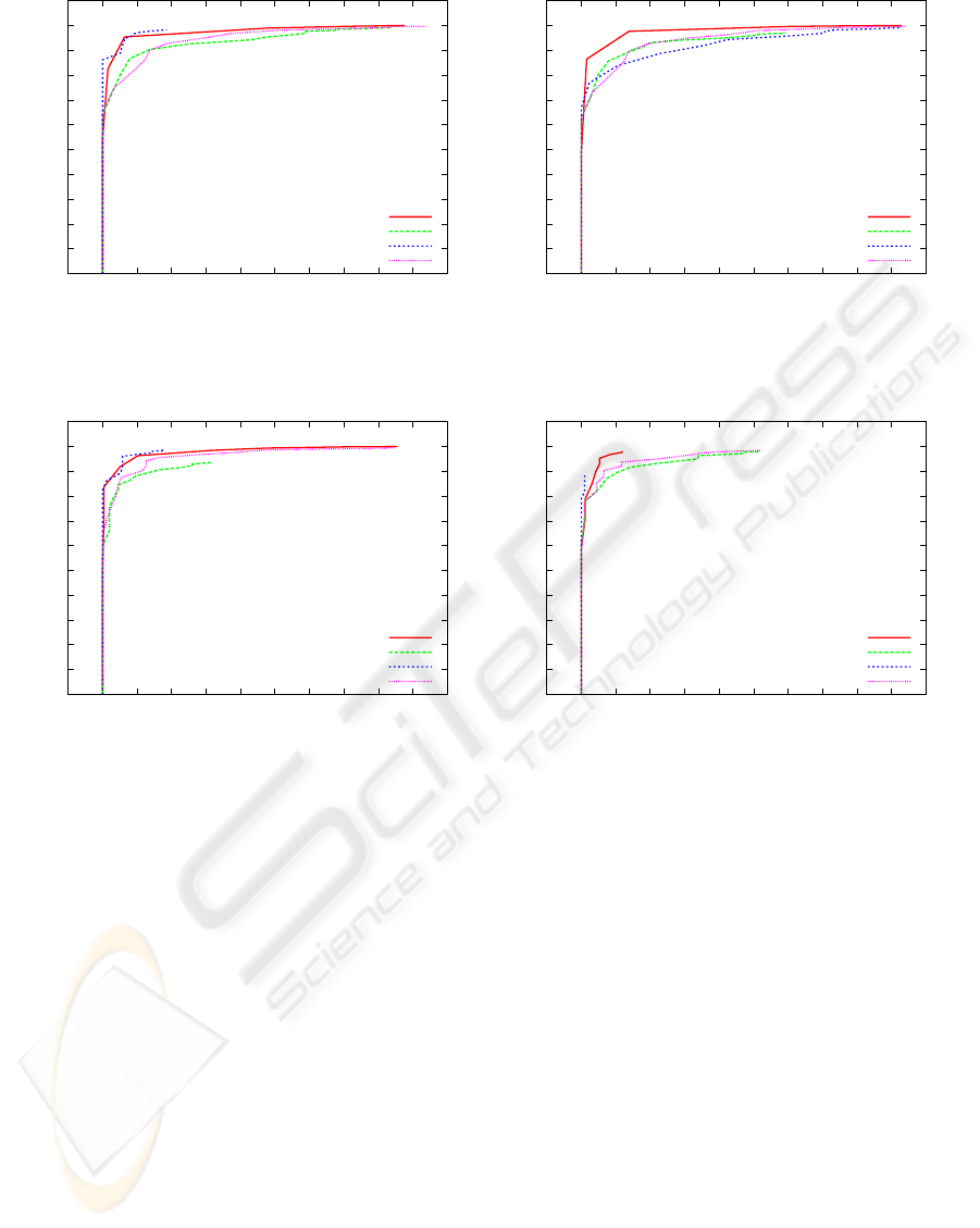
4.2 Robustness to Outliers

To evaluate the robustness to outliers in the train-

ing set, model learning was performed on a training

set containing 200.000 (20m rope) lines of rope data.

For learning, the view containing the most defects (9

defects) was chosen. Testing was performed on the

remaining three views, also containing each at least

seven defects. For comparison, the same experiment

was performed with a model, learned from 200.000

defect-free camera lines (20m rope). The resulting

ROC curves are compared in ﬁgure 6. The ROC curve

in ﬁgure 6(a) gives the averaged ROC for the model,

learned on defect-free training data. Figure 6(b) vi-

sualizes the results obtained with a model, learned

from a training set including outliers. Obviously, the

method is robust to few outliers in the training set,

as the results differ not signiﬁcantly from each other.

Where the LP features show the most robust behavior,

the LBP features seem to be error-prone if outliers are

contained in the training set. The size of the training

set was increased in the experiment, to incorporate as

many defects as possible.

4.3 Generalization Ability

For the evaluation of the generalization ability, learn-

ing was performed on a real, faultless rope, acquired

in a controlled environment. Testing on the other hand

was performed on different rope data from a real rope-

way containing defective regions. Both ropes belong

to the same construction type and they only differ in

their diameter by 10 pixels. In ﬁgure 7 the results are

depicted by the corresponding ROC curves, averaged

over all views. Figure 7(a) is generated by learning

and testing on the same rope from the ropeway and

ﬁgure 7(b) shows the result for learning in the con-

trolled setup and testing on real-life rope data. In both

VISAPP 2009 - International Conference on Computer Vision Theory and Applications

176

0.1

0.2

0.3

0.4

0.5

0.6

0.7

0.8

0.9

0 0.1 0.2 0.3 0.4 0.5 0.6 0.7 0.8 0.9 1

True Positive Rate

False Positive Rate

Co-occurrence

LBP

Irregularity

(a)

0.1

0.2

0.3

0.4

0.5

0.6

0.7

0.8

0.9

0 0.1 0.2 0.3 0.4 0.5 0.6 0.7 0.8 0.9 1

True Positive Rate

False Positive Rate

Co-occurrence

LBP

Irregularity

(b)

Figure 6: Comparison of ROC curves for learning with a defect-free training set (a) and a training set including defects (b).

0.1

0.2

0.3

0.4

0.5

0.6

0.7

0.8

0.9

0 0.1 0.2 0.3 0.4 0.5 0.6 0.7 0.8 0.9 1

True Positive Rate

False Positive Rate

Co-occurrence

LBP

Irregularity

(a)

0.1

0.2

0.3

0.4

0.5

0.6

0.7

0.8

0.9

0 0.1 0.2 0.3 0.4 0.5 0.6 0.7 0.8 0.9 1

True Positive Rate

False Positive Rate

Co-occurrence

LBP

Irregularity

(b)

Figure 7: Comparison of the ROC curves for learning and testing on the same data set (a) and learning and testing on two

different, identically constructed rope data sets (b).

cases the size of the learning set was 20.000 camera

lines (2m rope). The LBP features obviously show

the best generalization performance. The decreased

performance of the LP features again is caused by

a missed defect in one single view, which neverthe-

less was correctly discovered in the other views. Co-

occurrence features as well as irregularity-based fea-

tures show a surprising good generalization perfor-

mance. In general, these results indicate a quite good

generalization ability of the overall approach.

5 DISCUSSION AND OUTLOOK

We presented important and meaningful extensions

of our former work. The one-class classiﬁcation

approach for anomaly detection in wire ropes, pre-

sented in (Platzer et al., 2008), was extended by three

well-established features from the ﬁeld of textural

defect detection, and their performances were com-

pared. The results emphasize the necessity of context-

sensitive features for this challenging task. Although

all compared features result in a good performance,

the overall behavior of the context-sensitive features

is better. With the presented approach 70 till 90 per-

cent of the rope can be excluded from a reinspection

by a human expert and only a region of 10 cm around

a detected defect has to be re-examined again. Exper-

iments emphasizing the robustness and generalization

ability of the approach were presented. They pointed

out that a perfect, faultless training set is not essen-

tial for model learning. Especially from the practical

point of view, this is an important improvement, pre-

cisely because one cannot assure a completely defect-

free training set. With regard to the generalization

ability, the learned model was evaluated on real-life

rope data of different, individual ropes, which belong

to the same construction type. Results indicate a good

ROBUSTNESS OF DIFFERENT FEATURES FOR ONE-CLASS CLASSIFICATION AND ANOMALY DETECTION

IN WIRE ROPES

177

generalization ability of learned models with respect

to ropes, which are constructed in the same way. In

the context of practical applicability this is a remark-

able improvement, as it is a difﬁcult and time consum-

ing task to learn an individual model of the respective

rope previous to every detection run.

In future, the focus will be turned to the defect lo-

calization. Using not only context-sensitive features,

but also incorporating them into a context-based clas-

siﬁcation could lead to a further improvement of the

system. Interference between the different views, ac-

quired by the prototype system is also an interesting

point under investigation. For both problems, hidden

Markov models seem to be a good framework.

ACKNOWLEDGEMENTS

This research is supported by the German Research

Foundation (DFG) within the particular projects DE

735/6-1 and WE 2187/15-1.

REFERENCES

Bailey, D. (1993). Frequency domain self-ﬁltering for pat-

tern detection. In Proceedings of the ﬁrst New Zealand

Conference on Image and Vision Computing, pages

237–243.

Chen, C. H., Pau, L. F., and Wang, P. S. P., editors (1998).

The Handbook of Pattern Recognition and Computer

Vision (2nd Edition). World Scientiﬁc Publishing Co.

EN 12927-7 (2004). Safety requirments for cableways in-

stallations designed to carry persons. ropes. inspec-

tion, repair and maintenance. European Norm: EN

12927-7:2004.

Harlick, R. M., Shanmugam, K., and Dinstein, I. (1973).

Textural Features for Image Classiﬁcation. IEEE

Transactions on Systems, Man and Cybernetics,

3(6):610–621.

Hodge, V. J. and Austin, J. (2004). A Survey of Outlier De-

tection Methodologies. Artiﬁcial Intelligence Review,

22(2):85–126.

Iivarinen, J. (2000). Surface Defect Detection with

Histogram-Based Texture Features. volume 4197 of

Society of Photo-Optical Instrumentation Engineers

(SPIE) Conference Series, pages 140–145.

Kumar, A. and Pang, K. H. (2002). Defect Detection in

Textured Materials Using Gabor Filters. IEEE Trans-

actions on Industry Applications, 38(2):425–440.

M¨aenp¨a¨a, T., Turtinen, M., and Pietik¨ainen, M. (2003).

Real-time surface inspection by texture. Real-Time

Imaging, 9(5):289–296.

Makhoul, J. (1975). Linear Prediction: A Tutorial Review.

Proceedings of the IEEE, 63(4):561– 580.

Markou, M. and Singh, S. (2003). Novelty detection: a re-

view - part 1: statistical approaches. Signal Process-

ing, 83(12):2481 – 2497.

Moll, D. (2003). Innovative procedure for visual rope in-

spection. Lift Report, 29(3):10–14.

Ojala, T., Pietik¨ainen, M., and Harwood, D. (1996). A com-

parative study of texture measures with classiﬁcation

based on featured distributions. Pattern Recognition,

29(1):51–59.

Ojala, T., Pietik¨ainen, M., and M¨aenp¨a¨a, T. (2000). Gray

Scale and Rotation Invariant Texture Classiﬁcation

with Local Binary Patterns. In Proceedings of the

European Conference on Computer Vision (ECCV),

pages 404–420.

Platzer, E.-S., Denzler, J., S¨uße, H., N¨agele, J., and Wehk-

ing, K.-H. (2008). Challenging anomaly detection in

wire ropes using linear prediction combined with one-

class classiﬁcation. In Proceedings of the 13th Inter-

national Fall Workshop Vision, Modeling and Visual-

ization, pages 343–352.

Rabiner, L. and Juang, B.-H. (1993). Fundementals of

speech recognition. Prentice Hall PTR.

Rautkorpi, R. and Iivarinen, J. (2005). Shape-Based Co-

occurrence Matrices for Defect Classiﬁcation. In Pro-

ceedings of the 14th Scandinaian Converence on Im-

age Analysis (SCIA), pages 588–597.

Tajeripour, F., Kabir, E., and Sheikhi, A. (2008). Fabric De-

fect Detection Using Modiﬁed Local Binary Patterns.

EURASIP Journal on Advances in Signal Processing,

8(1):1–12.

Tax, D. M. J. (2001). One-Class classiﬁcation: Concept-

learning in the absence of counter-examples. Phd the-

sis, Delft University of Technology.

Varma, M. and Zisserman, A. (2003). Texture Classiﬁca-

tion: Are Filter Banks Necessary? In Proceedings of

the IEEE Conference on Computer Vision and Pattern

Recognition (CVPR), volume 2, pages 691–698.

Vartianinen, J., Sadovnikov, A., Kamarainen, J.-K., Lensu,

L., and K¨alvi¨ainen, H. (2008). Detection of irregular-

ities in regular patterns. Machine Vision and Applica-

tions, 19(4):249–259.

VISAPP 2009 - International Conference on Computer Vision Theory and Applications

178

REFERENCES

Bailey, D. (1993). Frequency domain self-filtering for pat-
tern detection. In Proceedings of the first New Zealand