MULTI-PERSPECTIVE PANORAMAS OF URBAN SCENES

WITHOUT SAMPLING ERRORS

Siyuan Fang and Neill Campbell

Department of Computer Science, University of Bristol, U.K.

Keywords:

Image Based Rendering, Multi-perspective panorama, City Visualization.

Abstract:

In this paper we introduce a framework for producing multi-perspective panoramas of urban streets from

a dense collection of photographs. The estimated depth information are used to remove sampling errors

caused by depth parallax of non-planar scenes. Then, different projections are automatically combined to

create the multi-perspective panorama with minimal aspect ratio distortions, which is achieved by a two-phase

optimization: ﬁrstly, the global optimal conﬁguration of projections is computed and then a local adjustment

is applied to eliminate visual artifacts caused by undesirable perspectives.

1 INTRODUCTION

Rendering a street usually needs to combine differ-

ent input photographs, as the ﬁeld of view of a sin-

gle photograph is limited to a portion of the street.

Traditional image mosaicing techniques (Szeliski and

Shum, 1997; Shum and Szeliski, 2000) assume in-

put images are captured at a single viewpoint. In

this case, the input images can be registered based

on certain alignment models, e.g., the homography.

However, it is usually impossible to place the view-

point far enough to encompass the entire street. To

acquire more scenes, we need to change the view-

point of the camera. Generating panoramas from im-

ages captured at different viewpoints is much more

challenging as an uniform alignment model for non-

planar scenes does not exist. In this paper, we present

a framework for constructing panoramas from image

sequences captured from a moving camera.

Recently, many approaches have been proposed

to combine images captured at different viewpoints

into a panoramic mosaic. These approaches can be

grouped into the following three categories:

View Interpolation. These approaches warp pix-

els from input images to a reference viewpoint us-

ing the pre-computed 3D scene structure (Chen and

Williams, 1993; Kumar et al., 1995). There are two

main problems with these approaches: to establish an

accurate correspondence between images for stereo is

still a hard vision problem, and there will likely be

holes in the result image due to sampling issues of the

forward mapping and the occlusion problem.

Optimal Seam. These approaches (Davis, 1998;

Agarwala et al., 2006) formulate the composition into

a labeling problem, i.e., pixel values are chosen to

be one of the input images. To avoid discontinuity,

the partition of different labeling is searched to min-

imize certain cost metrics such as pixel value differ-

ence. However, for scenes with large depth variations,

it is often impossible to ﬁnd such an optimal partition

that can create seamless mosaics.

Strip Mosaic. The basic idea of the strip mosaic

is to cut a thin strip from a dense collection of im-

ages and put them together to form a panorama. In

the push-broom model (Zhu et al., 2001; Zheng,

2003), the result image exhibits parallel in one direc-

tion and perspective in the other, while the crossed-

slits (Zomet et al., 2003) model is perspective in one

direction and is perspective from a different view-

point in the other direction. The aspect ratio dis-

tortion is inherent due to the different projections

along the two directions. Moreover, since the pin-

hole camera is used to capture input images, the re-

sult exhibits sampling errors due to the depth paral-

lax. By combining different projection models, multi-

perspective panoramas can be synthesized, e.g., (Ro-

man et al., 2004; Wexler and Simakov, 2005; Roman

and Lensch, 2006).

Our approach is based on the strip mosaic, as it

has many advantages. Strip mosaic are more efﬁcient

191

Fang S. and Campbell N. (2009).

MULTI-PERSPECTIVE PANORAMAS OF URBAN SCENES WITHOUT SAMPLING ERRORS.

In Proceedings of the Fourth International Conference on Computer Graphics Theory and Applications, pages 191-198

DOI: 10.5220/0001785101910198

 SciTePress

than view interpolation, and thus can be easily scaled

to long image sequences. Furthermore, unlike the op-

timal seam approach, even for scenes with complex

depth, strip mosaic can produce satisfactory results

by removing the sampling error and minimizing the

aspect ratio distortion. In general, we have made two

contributions:

1. We propose an approach for eliminating the sam-

pling error based on the 3D scene structure. The

principle behind our approach is similar to view

interpolation, but we only perform the “interpola-

tion” along one direction, and thus avoid the fore-

mentioned problems with the classic view inter-

polation techniques.

2. We present a two-phase optimization frame-

work to create the multi-perspective panorama.

Firstly, the optimal conﬁguration of projections is

searched to minimize the aspect ratio distortion.

Then, local adjustment is applied to eliminate ar-

tifacts caused by undesirable perspectives.

The rest of this paper is organized as: Section 2 in-

troduces the use of strip mosaic for rendering streets

and the sampling error. Section 3 presents our ap-

proach for eliminating sampling errors. Section 4

presents the framework for generating the optimal

multi-perspective panorama. Section 5 presents the

result and Section 6 concludes this paper.

2 STRIP MOSAIC AND THE

SAMPLING ERROR

In our system, street scenes are captured by a pre-

calibrated video camera mounted on a vehicle, which

is moving down a street with a slow and smooth speed

to capture it looking sideways. Strips are cut from the

captured image sequence and pasted into the result

image. From the plan view of the capturing setup,

each strip represents a sampled ray used to render

an image from a novel horizontal projection center,

which is actually a vertical slit in the 3D view. Figure

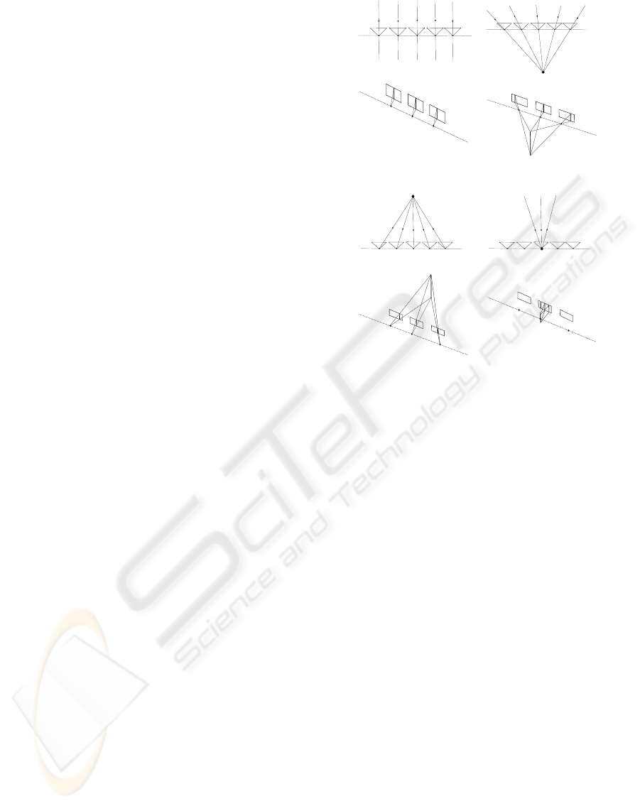
1 illustrates projection models relevant in our applica-

tion, which are four special cases of the general linear

camera summarized in (Yu and McMillan, 2004).

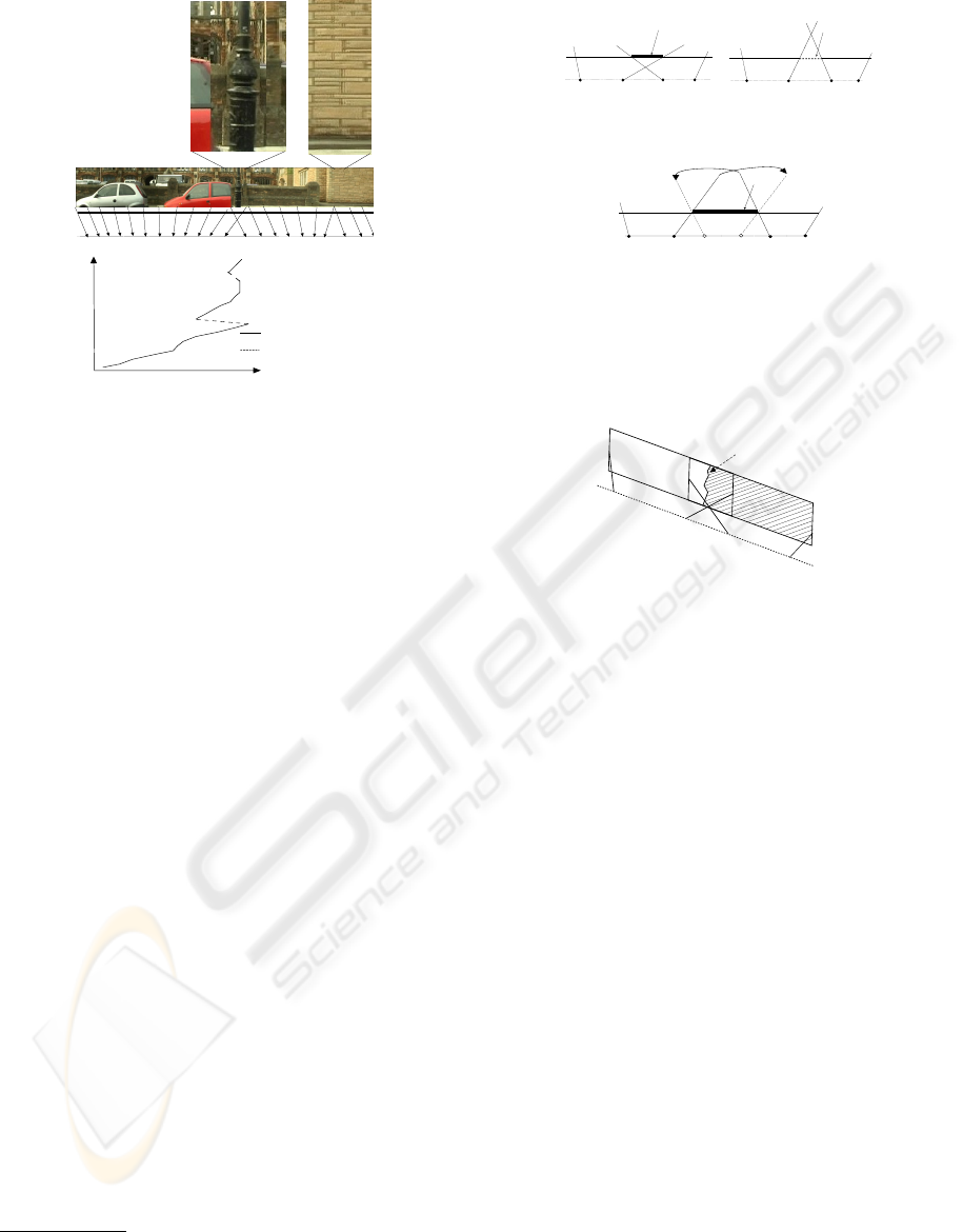
Because scenes within each strip are rendered

from a particular pinhole perspective, given a cer-

tain strip width, there is a depth at which scenes

show no distortion. For a further depth, some por-

tions of the surface might be duplicately rendered,

i.e., over-sampled, while for a closer depth, some por-

tions of the surface can not be fully covered, i.e.,

under-sampled. In the literature, this kind of artifact is

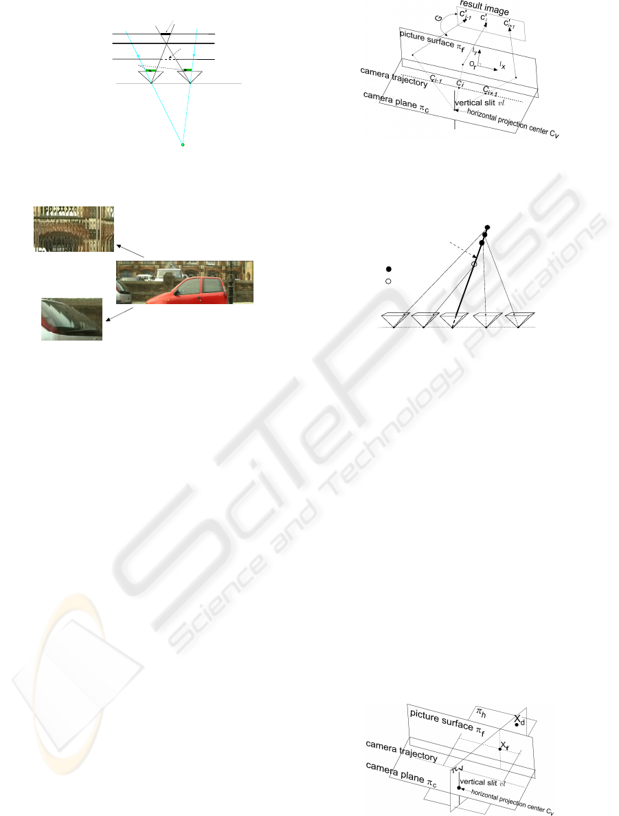
named the sampling error (Zheng, 2003). Figure 2(a)

camera trajectory

(a)

camera trajectory

vertical slit

camera trajectory

(b)

camera trajectory

vertical slit

camera trajectory

vertical slit

(c)

camera trajectory

vertical slit

camera trajectory

vertical slit

(d)

Figure 1: Projection Models. (a) The push-broom model,

where the horizontal projection center is placed at inﬁnity.

(b) The crossed-slits model, where the horizontal projection

center is placed off the camera trajectory. (c) The inverse

perspective, where the horizontal projection center is put

behind the camera trajectory. (d) The pinhole model, where

the horizontal projection center is just placed at a camera’s

optical center.

illustrates the sampling error and Figure 2(b) gives a

real example.

3 MOSAICING WITHOUT

SAMPLING ERRORS

3.1 Single Direction Interpolation

In our system, the mosaicing result is rendered on a

picture surface, which is deﬁned by a 3D plane π

We assume the camera trajectory lies on a plane π

If scenes are exactly located on the picture surface, a

point of the result image (p

, q

) can be mapped to a

point (p, q) of an input frame by a projective transfor-

mation, i.e., the homography:









= H









= P









(1)

where P

= KR

[I | −C

] is the camera matrix of the i

GRAPP 2009 - International Conference on Computer Graphics Theory and Applications

192

vertical slit

under-sampled

non-distortion depth

over-sampled

strip width

camera trajectory

(a)

over-sampled

under-sampled

(b)

Figure 2: The Sampling Error (a) The sampling error is

caused by the depth parallax. (b) A real example of the

sampling error.

frame. The camera parameters are extracted from the

video sequence by the structure-from-motion (SFM)

algorithm (Hartley and Zisserman, 2004). G is a 4 × 3

matrix that establishes the mappings between a 2D

point of the result image and a 3D point on the picture

surface.

We assume the horizontal projection center C

lies

on the camera plane and the vertical slit vl is the line

that passes through C

and perpendicular to the cam-

era plane. We project the camera center C

onto the

result image c

along the line connecting C

and C

see Figure 3. A given point of the result image is

rendered with the frame corresponding to the closest

camera center projection c

For scenes with complex depth structures, a pixel

from the input frame should be warped onto the result

image based on the actual 3D coordinate, which is es-

timated by an approach resembling that in (Goesele

et al., 2006). We search along the back-projected ray

of a pixel and for each depth h, we project the cor-

responding 3D coordinate onto a neighboring frame

and compute the normalized cross-correlation (NCC).

The 3D coordinate is that with the highest NCC score.

To enforce multi-view consistency, we compute the

average value of h in a set of neighboring frames and

use the robust estimation (RANSAC) to remove out-

Figure 3: The mosaic is rendered on the picture surface.

Camera centers are projected onto the picture surface and

then mapped to the ﬁnal result image.

i-1

i-2

i+1

i+2

i, i-1

i, i+1

i, i+2

i, i-2

back-projected ray

inliner

outliner

Figure 4: 3D Scene coordinate reconstruction.

liers. Figure 4 illustrates the depth estimation ap-

proach.

We deﬁne a vertical center line CL

that passes

on the result image. A vertical boundary line

{i↔i+1}

is drawn between any consecutive camera

center projections. The center line CL

is then mapped

on the source frame I

. For each individual

pixel (p, q), suppose its corresponding 3D coordinate

is X

, its mapping onto the picture surface is the inter-

section of 3 planes: the picture surface π

, the plane

that contains X

and the vertical slit vl and the

plane π

that contains X

and the tangent line of the

camera trajectory at C

on the camera plane, see Fig-

ure 5. Once the intersection is recovered, it is mapped

to the result image by G

, the pseudo-inverse of G.

For a given input frame I

, we only examine pixels

within a region around

. For each row of I

, we

take the pixel on

as the starting point and search

Figure 5: A pixel from the input frame is warped to the

picture surface based on its corresponding 3D coordinate.

MULTI-PERSPECTIVE PANORAMAS OF URBAN SCENES WITHOUT SAMPLING ERRORS

193

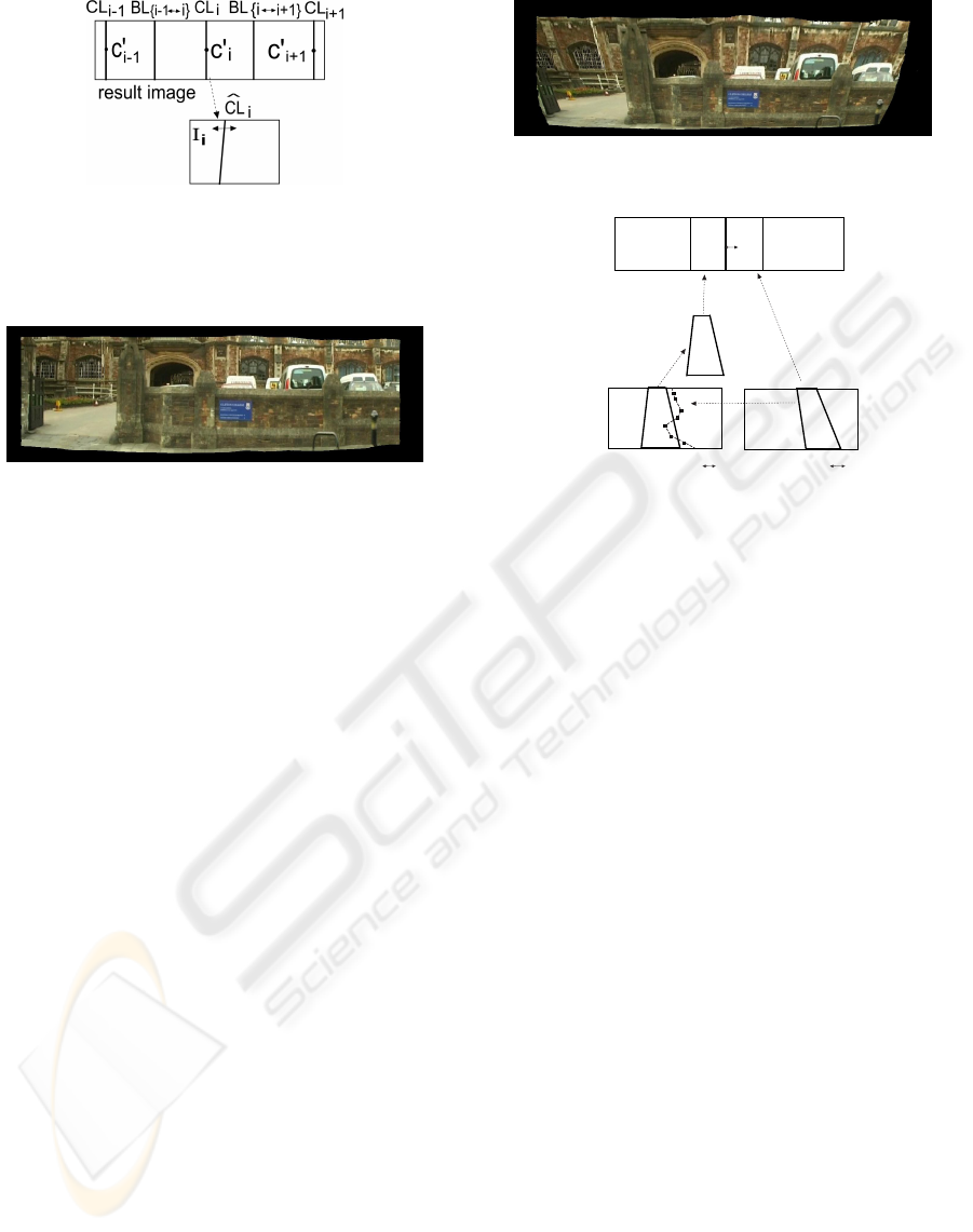
Figure 6: The center lines and boundary lines on the re-

sult image. The center line is mapped to the correspond-

ing frame. The pixel warping is carried out within a region

around the center line mapping.

Figure 7: The rendered image without sampling errors.

into both sides, once the warped point onto the re-

sult image is beyond the boundary line BL

{i↔i+1}

{i−1↔i}

, we proceed to the next row, see Figure 6.

However, this approach is sensitive to incorrect

depth estimations. In practice, we assume the X-axis

of the camera is coincident with the tangent line of

the camera trajectory. Therefore, the value of q

can

be directly computed using the homograph H

. On the

other hand, the value of p

depends on the actual 3D

coordinate of (p, q). Suppose the picture surface π

intersects π

at a 3D line, and X

and X

are two points

on that 3D line, then its mapping onto the result image

is deﬁned as:







((G

)

)((G

)

) − ((G

)

)((G

)

((G

)

)((G

)

) − ((G

)

)((G

)

((G

)

)((G

)

) − ((G

)

)((G

)



















= 0

(2)

where (G

)

denotes the k

row of the matrix G

By solving this equation, the value of p

can be de-

rived. Because with one direction the pixel warping

adopts the original projective transformation, while

the other is based on the real 3D coordinate, we name

our rendering strategy a “single direction interpola-

tion” as opposed to the full perspective interpolation.

Figure 7 shows a rendered result.

In principle, the picture surface should lie along

the dominant plane of street scenes, such as the build-

ing facet. One can ﬁt the plane equation of the picture

surface to the 3D points discovered by the SFM al-

gorithm. However the ﬁtting result is often a slanted

plane, which would cause an non-uniform scaling of

Figure 8: The result image is rendered on a slanted picture

surface.

i+1

{ i

i+1}

i+1

i+1,{ i

i+1}

i,{ i

i+1}

matched points

row based warping

result image

i+1

Figure 9: The fast algorithm using depth-variant strips.

scenes, see Figure 8. Therefore, we choose the pic-

ture surface to be perpendicular to the camera plane

and parallel with the camera trajectory, i.e., fronto-

parallel. Based on this constraint, we use the least

square ﬁt to ﬁnd its plane equation.

3.2 A Fast Approximation

It is very costly to compute the actual 3D coordinate

for every warped pixel, and for large texture-less area,

the depth estimation is not reliable. Therefore, we

implement a fast approximation. Assuming

and

i+1

are mappings of the center line CL

and CL

i+1

and

i,{i↔i+1}

and

i+1,{i↔i+1}

are mappings of the

boundary line BL

{i↔i+1}

from the result image onto

two consecutive frames I

and I

i+1

, see Figure 9. We

search along the line

i+1,{i↔i+1}

and match a set of

corresponding points on I

with high NCC values. By

interpolating and extrapolating these matched points,

a curved stitching line is deﬁned on I

. We warp each

row based on this stitching line, then the new derived

quadrilateral is transformed to the result by H

. On the

other hand, the quadrilateral encompassed by

i+1

and

i+1,{i↔i+1}

on I

i+1

is directly transformed to

the result image by H

i+1

. The illustration is presented

in Figure 9.

GRAPP 2009 - International Conference on Computer Graphics Theory and Applications

194

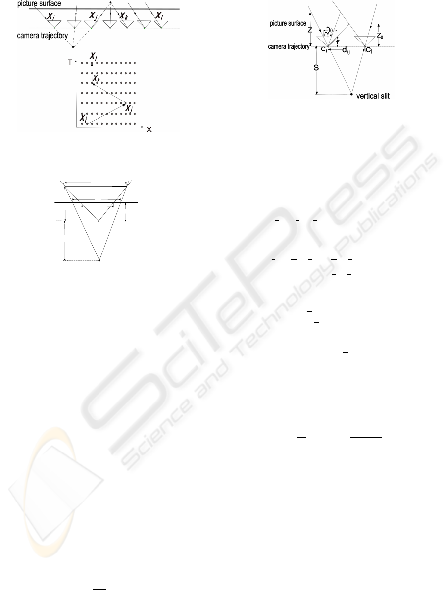
Figure 10: The multi-perspective panorama and the path on

the X-T space.

vertical slit

Figure 11: The aspect ratio distortion.

4 MULTI-PERSPECTIVE

PANORAMAS

4.1 Global Optimization

This section describes how the projection models

listed in Figure 1 are automatically combined to cre-

ate a multi-perspective panorama. According to the

paradigm proposed by Wexler and Simakov (Wexler

and Simakov, 2005), the transitions of the strip loca-

tion for creating a panorama form a path through the

X-T space of the stacked volume of frames. To adopt

this paradigm, the camera trajectory is restricted to

be linear, i.e., straight. The picture surface is chosen

to be fronto-parallel. In this setup, given a particular

horizontal projection center, the center line CL

in the

result image is mapped to a vertical line

in I

, so

that its X-direction location is ﬁxed across rows. We

denote this location as x

. For illustration see Figure

10.

Figure 11 shows the aspect ratio distortion in this

case, deﬁned by:

α =

s+z

z(z

+ s)

(z + s)

(3)

To search the optimal path, we need a proper cost

Figure 12: The relationship between the aspect ratio distor-

tion and strip width.

metric for strip transition. The fast approximation

algorithm gives us an intuition that the warping rate

of a row reﬂects the aspect ratio distortion in the re-

sult. As shown in Figure 12, if scenes are exactly

located on the picture surface the strip width γ

is:

i j

(

), while for off-plane scenes, the strip

width γ is:

i j

(

). The rate between γ

and γ

is equal to the aspect ratio distortion:

i j

(

)

i j

(

)

z(z

+ s)

(z + s)

= α (4)

Based on (4), we deﬁne our error metric as:











−1k

max(k

k,1)

≤ x

−x

−1k

max(k

k,1)

> x

(5)

A backward edge (x

> x

), corresponds to an inverse

perspective, see Figure 1(c). We penalize this with

a higher cost η

−x

, and η ≈ 1.2. Based on this

error metric, the cost function associated with a strip

transition is deﬁned as:

E =

(

∑

) + β

− x

i j

(6)

We only consider warping rates of rows with those

matched points rather than the entire strip. p denotes

such a matched point and n

denotes the number of

matched points involved. The second term of (6) is

used to suppress strips that are too wide, because in

this case discontinuities at strip borders are likely to

be visible. Dijkstra’s algorithm is used to ﬁnd the

shortest path. After the optimal projection conﬁgu-

ration is achieved, we use the fast approximation al-

gorithm to create the sampling-error-free panorama.

We ﬁrst search along the optimal path to locate all

the maximal connected forward segments and render

the result with these forward segments. Then the re-

maining backward segments are processed. Figure

13 presents an example, where some portions exhibit

MULTI-PERSPECTIVE PANORAMAS OF URBAN SCENES WITHOUT SAMPLING ERRORS

195

Forward Segment

Backward Segment

Figure 13: The result of the global optimization and the

corresponding optima path.

heavy artifacts caused by the backward segment. In

the next section, we describe how this problem can be

handled by a local adjustment step.

4.2 Local Adjustment

The idea of the local adjustment is to avoid the use

of the inverse perspective (the backward segments),

i.e., we only consider those forward segments. For

simplicity, we use the term “virtual camera” to de-

note these forward segments

. There are two possi-

ble spatial relationships between two adjacent virtual

cameras: their rendered areas overlap on the picture

surface Figure 14(a), or disjoint Figure 14(b). For

the latter, we need to extend the ﬁeld of view of the

two virtual cameras to make them overlap, see Figure

14(c).

To make a seamless composition, we divide the

overlapping region of the two adjacent virtual cam-

eras into two parts, each of which is labeled with

pixel values from the rendered result of a single vir-

tual camera, see Figure 15. The optimal partition can

be cast into a graph cut problem. We deﬁne the cost

of a cut between any two neighboring pixels p and q

as:

C(p, q) = C

(p, q) + µC

(p, q) (7)

(p, q) is the pixel value difference and C

(p, q)

measures the partition cost in the gradient domain.

The weight µ is chosen to be 0.01. C

(p, q) is deﬁned

It should be noted that the term virtual camera is only

used to denote forward segments, in fact, as shown in Fig-

ure 13, they are usually composed of several different pro-

jections.

start

end

start

end

overlapping region

(a)

start

end

start

end

empty region

(b)

start

end

start

end

overlapping region

end

start

(c)

Figure 14: The Spatial relationship between adjacent vir-

tual cameras. (a) Overlapping. (b) Disjoint. (c) The disjoint

virtual cameras are expanded based on the bordering pro-

jection direction.

partition line

start

end

start

end

Figure 15: The Optimal Partition.

as:

(p, q) =

∑

channel s

(NSSD(R

, R

, ω(p))+

NSSD(R

, R

, ω(q)))

(8)

where R

and R

denote the rendered images of the

two virtual cameras A and B. NSSD(R

, R

, ω(p))

is the normalized sum of squared pixel value differ-

ence between R

and R

computed in a patch around

a given pixel (ω(p)).

The gradient partition cost is the sum of two terms

measuring the gradient magnitude and similarity:

(p, q) = M

(p)+ M

(q) + M

(p)+ M

(q) +

∑

l∈{x,y}

(k∇

(p)− ∇

(p)k +

k∇

(q) − ∇

(q)k)

(9)

where M

(p) denotes the magnitude of the gradient

at a pixel, and k∇

· k denotes the gradient along one

dimension of the image space, x or y. We choose the

weight ρ = 0.8.

The graph cut problem is solved using the max-

ﬂow/min-cut algorithm described in (Boykov and

Kolmogorov, 2004). Figure 16 presents the improved

panorama of Figure 13. In addition, a given portion

of the picture surface might be covered by more than

two virtual cameras. We adopt a straightforward so-

lution: virtual cameras are processed in a series and

for each incoming virtual camera, the optimal parti-

GRAPP 2009 - International Conference on Computer Graphics Theory and Applications

196

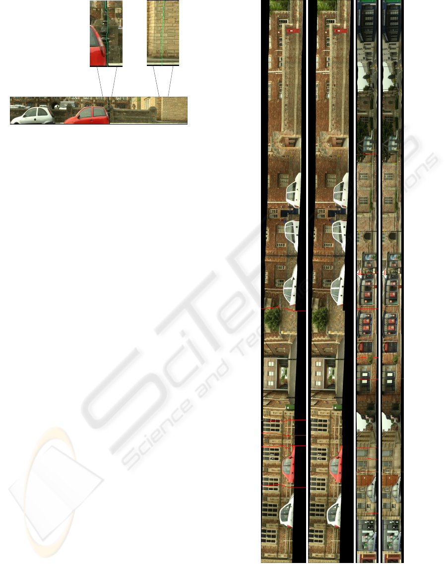
Figure 16: The multi-perspective image after local adjust-

ment. The zoom-in view shows the optimal partition line

(seam).

tion is performed on overlapping region between the

current virtual camera and areas already rendered on

the picture surface. If the incoming virtual camera has

no overlapping region with areas so far rendered, the

new virtual camera and its immediately previous one

are expanded.

5 RESULTS

We have conducted experiments on our frame-

work using image sequences captured by a digi-

tal video camcorder (Canon XM1), which captures

at 25 frames/second. Compared to existing multi-

perspective panorama generation techniques, e.g.,

(Wexler and Simakov, 2005; Roman and Lensch,

2006), the essential improvement of our approach lies

in the local adjustment as it makes our system capable

of achieving the best trade-off between the seamless

result and the maximal preservation of the human-eye

perspective. Approaches described in (Wexler and

Simakov, 2005; Roman and Lensch, 2006) are equiv-

alent to the global-optimization step in our frame-

work. In this sense, results with and without the local

adjustment shown in Figure 13 and 16 present a com-

parison between these two kinds of approaches.

We have applied our techniques to longer streets.

The result in Figure 17(a) visualizes a street that spans

around 80 meters, and the street visualized in Figure

17(b) spans around 160 meters.

For the mosaicing result in Figure 7, the cam-

era pose is extracted by Voodoo camera tracker

[http://www.digilab.uni-hannover.de/docs/manual.html]

with bundle adjustment. For long streets shown

in Figure 16, 17(a) and 17(b), we rectify the input

sequence to compensate for the camera tilt and we

assume a translational motion along the horizontal

direction at a constant speed. While, along the

(a) (b)

Figure 17: Multi-perspective panoramas. The ﬁrst row of

each image set shows the partition seam and the second

without.

MULTI-PERSPECTIVE PANORAMAS OF URBAN SCENES WITHOUT SAMPLING ERRORS

197

vertical direction, the displacement is computed by

matching salient features and RANSAC is used to

remove outliers.

The optimization framework is tested on a PC

with two Xeon CPUs (2.00 GHz and 1.99 GHz) and

1.50GB ram. The global optimization of the result in

Figure 17(a) (with 980 482 × 429 input frames) takes

around 12 minutes and the result in Figure 17(b) (with

1200 395 × 227 input frames) takes around 8 minutes

. The local adjustment of these two results both takes

around 4 minutes.

6 CONCLUDING REMARKS

This paper presents a framework for producing multi-

perspective panoramas of street scenes. Our approach

uses an estimation of 3D scene structure to eliminate

the sampling error caused by the depth parallax. Then

an automatic optimization is performed to create the

panorama with minimal aspect ratio distortions. Af-

ter that, a further local adjustment step is applied to

remove artifacts caused by inverse perspectives. In

principle, our approach is restricted to straight cam-

era trajectories and approximately fronto-parallel pic-

ture surfaces. For non-straight camera trajectories, we

assume they are piece-wise linear. However, for tra-

jectories with abrupt direction changes, although our

rendering system can handle this situation, the result

of our global optimization is not theoretically accu-

rate, as the aspect ratio distortion in this case is not

yet clear.

REFERENCES

Agarwala, A., Agrawala, M., Cohen, M., Salesin, D., and

Szeliski, R. (2006). Photographing long scenes with

multi-viewpoint panoramas. ACM Transactions on

Graphics, 25(3):853 – 861.

Boykov, Y. and Kolmogorov, V. (2004). An experimental

comparison of min-cut/max-ﬂow algorithms for en-

ergy minimization in vision. IEEE Transactions on

Pattern Analysis and Machine Intelligence, 26:1124–

1137.

Chen, S. and Williams, L. (1993). View interpolation

for image synthesis. Computer Graphics, 27(Annual

Conference Series):279–288.

Davis, J. (1998). Mosaics of scenes with moving objects.

In Proceedings of the IEEE Conference on Computer

Vision and Pattern Recognition, pages 354–360.

To eliminate the redundant computation of matching

points, a dense disparity map for each consecutive frame

pair is pre-computed before optimization.

Goesele, M., Curless, B., and Seitz, S. (2006). Multi-view

stereo revisited. In Proceedings of IEEE Conference

on Computer Vision and Pattern Recognition, pages

2402–2409.

Hartley, R. and Zisserman, A. (2004). Multiple view geom-

etry in computer vision. Cambridge University Press,

2 edition.

Kumar, R., Anandan, P., Irani, M., Bergen, J., and Hanna,

K. (1995). Representation of scenes from collections

of images. In Proceedings of IEEE Workshop on Rep-

resentation of Visual Scenes, pages 10–17.

Roman, A., Garg, G., and Levoy, M. (2004). Interactive

design of multi-perspective images for visualizing ur-

ban landscapes. In Proceedings of IEEE Visualization,

pages 537–544.

Roman, A. and Lensch, H. (2006). Automatic multiper-

spective images. In Proceedings of 17th Eurographics

Symposium on Rendering, pages 161–171.

Shum, H. and Szeliski, R. (2000). Construction of

panoramic image mosaics with global and local align-

ment. International Journal of Computer Vision,

36(2):101–130.

Szeliski, R. and Shum, H. (1997). Creating full view

panoramic image mosaics and environment maps. In

Proceedings of SIGGRAPH 97, Computer Graphics

Proceedings, Annual Conference Series, volume 31,

pages 251–258.

Wexler, Y. and Simakov, D. (2005). Space-time scene man-

ifolds. In Proceedings of the International Conference

on Computer Vision, volume 1, pages 858 – 863.

Yu, J. and McMillan, L. (2004). General linear cameras.

In Proceedings of European Conference on Computer

Vision, pages 14–27.

Zheng, J. (2003). Digital route panoramas. IEEE Multime-

dia, 10(3):57– 67.

Zhu, Z., Riseman, E., and Hanson, A. (2001). Parallel-

perspective stereo mosaics. In Proceedings of the

International Conference on Computer Vision, vol-

ume 1, pages 345–352.

Zomet, A., Feldman, D., Peleg, S., and Weinshall, D.

(2003). Mosaicing new views: The crossed-slits pro-

jection. IEEE Transactions on Pattern Analysis and

Machine Intelligence, 25(6):741– 754.

GRAPP 2009 - International Conference on Computer Graphics Theory and Applications

198