A SVD BASED IMAGE COMPLEXITY MEASURE
David Gustavsson, Kim Steenstrup Pedersen and Mads Nielsen
Department of Computer Science, University of Copenhagen , Universitetsparken 1, DK-2100 Copenhagen, Denmark
Keywords:
Image complexity measure, Geometry, Texture, Singular value decomposition, SVD, Truncated singular value
decomposition, TSVD, Matrix norm.
Abstract:
Images are composed of geometric structures and texture, and different image processing tools - such as
denoising, segmentation and registration - are suitable for different types of image contents. Characterization
of the image content in terms of geometric structure and texture is an important problem that one is often faced
with. We propose a patch based complexity measure, based on how well the patch can be approximated using
singular value decomposition. As such the image complexity is determined by the complexity of the patches.
The concept is demonstrated on sequences from the newly collected DIKU Multi-Scale image database.
1 INTRODUCTION
Images contain a mix of different types of informa-
tion, from highly stochastic textures such as grass and
gravelto geometric structures such as houses and cars.
Different image processing tools are suitable for dif-
ferent type of image contents and most tools are very
image content dependent. The definition of what is
texture and geometry is not particularly agreed upon
in the computer vision community. Our hypothesis
is that the separation between geometry and texture
is defined through the purpose of the method and the
scale of interest. What may be considered an unim-
portant structure / texture in one application may be
considered important in another.
For example, segmentation of an image contain-
ing objects with clear geometric structures forming
boundaries calls for edge-based or geometry-based
methods such as watersheds (Olsen and Nielsen,
1997), the Mumford-shah model (Mumfordand Shah,
1985), level sets (Sethian, 1999), or snakes (Kass
et al., 1988). While segmentation of an image con-
taining objects only discernable by differences in tex-
ture calls for texture based segmentation methods
(Randen and Husoy, 1999). That is, the type of ob-
jects we are attempting to segment defines our scale
of interest, i.e. what type and scale of structure we
include in the model of a segment.
In denoising an image containing geometric struc-
tures calls for e.g. an edge preserving method such as
anisotropic diffusion (Weickert, 1998) or total varia-
tion image decomposition (Rudin et al., 1992). For
images containing small scale texture, a patch based
denoising method such as non-local mean filtering
may be more appropriate (Buades et al., 2008). Again
we see that depending on the purpose we include
structures at finer scales into the model of the prob-
lem as needed.
As a final example, we mention that total varia-
tion (TV) image decomposition, and other functional
base methods, are very successful for inpainting im-
ages containing geometric structures (Chan and Shen,
2005). Unfortunately the functional based methods
fails to faithfully reconstruct regions containing small
scale structures, however texture based methods man-
age to reconstruct such images (Efros and Leung,
1999; Criminisi et al., 2004; Gustavsson et al., 2007;
Cuzol et al., 2008). In the functional approaches the
focus is solely on large scale structures or geometry,
whereas in the texture methods small scale texture is
included in the model.
Prior knowledge about the methods and the image
content are therefore essential for successfully solv-
ing a task. A natural question is: ”For a given type of
images, which type of methods are suitable?” Often
one wants to characterize the methods by analyzing
the type of images that it is (un)suitable for. To be
able to characterize the methods in this way, the im-
ages must be characterized with respect to the image
contents. An image complexity measure is needed,
i.e. a measure that quantify the image contents with
respect to geometric structure and texture or scale of
interest.
A patch based complexity measure using Singular
34
Gustavsson D., Steenstrup Pedersen K. and Nielsen M. (2009).
A SVD BASED IMAGE COMPLEXITY MEASURE.
In Proceedings of the Fourth International Conference on Computer Vision Theory and Applications, pages 34-39
DOI: 10.5220/0001785400340039
Copyright
c
 SciTePress

Value decomposition (SVD) is presented. The com-
plexity for the patch is determined by the number of
singular values that are required for good approxima-
tion - the matrix rank of a good approximation. The
number of singular values that are required for ap-
proximating an image patch is used for characteriz-
ing the patch content. The global complexity measure
for the image is computed as the mean complexity of
all patches in the image. The proposed complexity
measure is evaluated on the baboon image and on the
newly collected DIKU Multi-Scale image sequence
database.
2 COMPLEXITY MEASURE
In the following section images are viewed as matri-
ces, hence the image complexity measure transforms
into a matrix complexity measure. Basic matrix prop-
erties are used extensively in the following section,
which can be found in e.g. (Golub and Loan, 1996).
One obvious approach is to approximate a matrix A
with a simpler matrix A
k
and measure the error (resid-
ual) between the original matrix A and the approxima-
tion A
k
. Here k is a parameter used for computing the
approximation A
k
. We assume that, as the parameter
k increases the error between A and A
k
decrease (or
at least not increase) and as k → ∞ the error becomes
0. The approximation A
k
should also be simpler than
A. To be able to use this approach, an error measure
between matrices and a matrix complexity measure
must be defined.
2.1 Error Measure - Matrix Norms
To measure the difference between the original im-
age A and a simpler approximation A
k
of I, it is nat-
ural to use a matrix norm kA− A
k
k. One of the most
commonly used matrix norms is the Frobenius norm
(which corresponds to the L
2
-norm). Let A be a m×n
matrix with elements a
ij
, the Frobenius norm of A is
defined as
kAk
F
= (
n
∑
j=1
m
∑
i=1
|a
ij
|
2
)
1
2
. (1)
Another common type of matrix norms are the so-
called induced matrix norms. Let A be a m× n ma-
trix and x ∈ R
n
a colon vector (i.e x = (x
1
, ··· ,x
n
)
T
),
the matrix norm induced by the vector norm kxk is
defined as
kAk = sup
kxk=1
kAxk
kxk
(2)
(or in words the smallest number α such that
kAxk
kxk
≤ α
for all x). The matrix norm is here defined in terms of
a vector norm kxk. The induced matrix norm can be
viewed as how much the matrix A expands the vec-
tors and is actually an operator norm. Different vector
norms can be used to induce different matrix norms,
most common are the p-norms defined as
kxk
p
= (
n
∑
i=1
| x
i
|
p
)
1
p
(3)
and especially the 2-norm kxk
2
= (x
T
x)
1
2
. The matrix
norm induced by the 2-norm is
kAk
2
= sup
kxk
2
=1
kAxk
2
kxk
2
(4)
Both the The Frobenius matrix norm and the matrix
2-norm are invariant under orthogonal transformation
and will be used in the following sections.
2.2 Matrix Complexity Measure -
Matrix Rank
Given a matrix A, a simpler matrix approximation A
k
of A should be constructed. But first one must define
what ’simpler’ means. A natural approach to quan-
tify complexity of a matrix is by the rank of the ma-
trix, and a simpler approximation of a matrix can be
viewed as a matrix with lower rank.
Let A be a m × n matrix then the rank of A can be
viewed as the dimension of the subspace spanned by
the columns of A = (a
1
, ··· ,a
n
),
rank(A) = dim( span{a
1
, ··· ,a
n
} ). (5)
2.3 Optimal Rank k Approximation
It is well known from matrix theory that a m× n ma-
trix A can be decomposed into
A = UΣV
T
(6)
where U is a m × m orthogonal matrix, V is a n × n
orthogonal matrix and Σ is a m × n diagonal matrix
with elements σ
1
, ··· ,σ
l
where l = min{m, n}. This
is the so-called Singular Value Decomposition (SVD),
where the σ
i
:s are called singular values and the col-
umn vectors u
i
and v
i
, of U and V are called sin-
gular vectors. The entries in Σ is ordered such that
σ
1
≥ σ
2
≥ ··· ≥ σ
l
≥ 0.
Using the fact that the Frobenious norms are invariant
under multiplication by orthogonal matrices gives
kAk
2
F
= kΣk
2
F
=
l
∑
i=1
(σ
i
)
2
. (7)
A SVD BASED IMAGE COMPLEXITY MEASURE
35

Let Σ
k
be the m × n matrix containing the k largest
singular values on the diagonal and let
A
k
= UΣ
k
V
T
. (8)
A
k
is the so-called Truncated Singular Value Decom-
position (TSVD) approximation of A where the first
k singular values are used, and if rank(A) ≥ k then
rank(A
k
) = k. The image approximation residual is
defined as A − A
k
and if, again, rank(A) ≥ k then
rank(A− A
k
) = rank(A) − k.
The reconstruction error or the residual error for the
Frobenious norm is
kA− A
k
k
F
= (
l
∑
i=k+1
(σ
(i)
)
2
)
1
2
(9)
and for the 2-norm
kA− A
k
k
2
= σ
k+1
. (10)
The rank(A
k
) ≤ rank(A), so A
k
is simpler in the sense
that its’ rank is not larger (and usually the rank is
lower). Furthermore A
k
is the best rank − k approxi-
mation of A in the sense that
A
k
= arg min
rank(B)=k
kA− Bk
2
(11)
So any matrix B with rank k has at least as large re-
construction error using the 2-norm as A
k
. A
k
is also
the best rank k approximation using the Frobenious
norm. Singular Value Decomposition can be viewed
as a method for finding the optimal basis and is re-
lated to other optimal basis methods such as Indepen-
dent Component Analysis (ICA) (Hyv¨arinen, 1999)
and Karhunen-Lo´eve Expansion (Kirby, 2000).
There are two possibilities to compare images by
comparing the norm of the residual. Either the num-
ber of singular values, k, are fixed and the reconstruc-
tion error kA
k
− Ak using k singular values are com-
pared. The other possibility is to keep the reconstruc-
tion error fixed, σ
err
, and use as many singular val-
ues that are required for the reconstruction error to be
lower than σ
err
. Either the rank k or the reconstruc-
tion error σ
err
is kept fixed.
Let k
0
be the number of singular values that should be
used in the reconstruction. The residual error (using
either the 2-norm or Frobenious norm) is
kA− A
k
0
k = σ
err
k
0
(12)
and σ
err
k
0
is called the singular value reconstruction er-
ror using k
0
singular values.
Let σ
err
be a fixed reconstruction error and let k be the
smallest integer such that
kA− A
k
k ≤ σ
err
(13)
k is called the singular value reconstruction index
(SVRI) at level σ
err
. The SVRI state the smallest
number of singular values that are required to get a re-
construction with a reconstruction error smaller than
σ
err
.
2.4 Global Measure
Instead of computing an approximation of the full im-
age, which is not feasible for high resolution images,
a patch based approach is adopted. The singular value
reconstruction error at level σ
err
is computed for each
p× p patch in the image.
Based on the patch complexities an image complexity
measure should be computed. The obvious candidate
is the mean or the mode complexity computed over
all patches in the image. The mean patch complex-
ity is used as the complexity measure for the image.
The interpretation of the mean, is simply the average
number of singular values that are required for an ap-
proximation, such that the reconstruction error is less
than σ
err
, of the patches in the image.
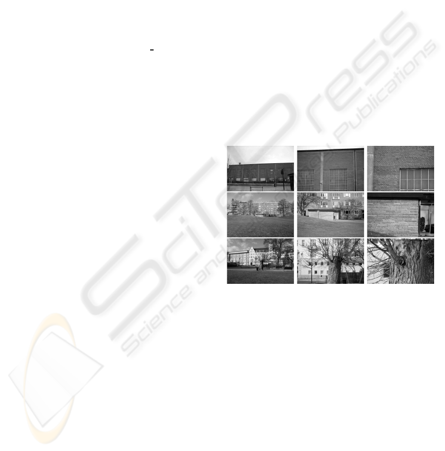
Figure 1: Image sequences - 02, 05 and 08 - from the DIKU
Multi- Scale image database (used in the experiments) at
three capture scales.
3 DIKU MULTI-SCALE IMAGE
DATABASE
The newly collected DIKU Multi-Scale image
database (Gustavsson et al., 2009), contains se-
quences of the same scene captured using varying fo-
cal length - called capture scales -, will be used to
analyze the distribution of singular values in natu-
ral image patches and analyze how the image content
changes over different capture scales.
The database contains sequences of natural images
- both man-made and natural environment - with a
large variety of scenes and distances to the main ob-
ject in the scene. Each sequence contains 15 high res-
VISAPP 2009 - International Conference on Computer Vision Theory and Applications
36

olution images of the same scene captured using dif-
ferent focal length. The zoom factor is roughly 16x
and the naming convention is that image 1 is the least
zoomed and 15 the most zoomed. Three examples of
sequences are shown in figure 1.
Furthermore, the part of the scene that is present at
all capture scales has been extracted, resulting in a se-
quence of region containing the same part of scene
captured at different capture scales. The part of the
scene present in the image to the right in figure 1,
has been extracted from the remaining 14 images (of
which two are shown in the figure).
Three sequences - 02 building with windows, 05
building without windows and 08 tree trunk - shown
in figure 1 are used in the experiments. The image
contents are very different on the different capture
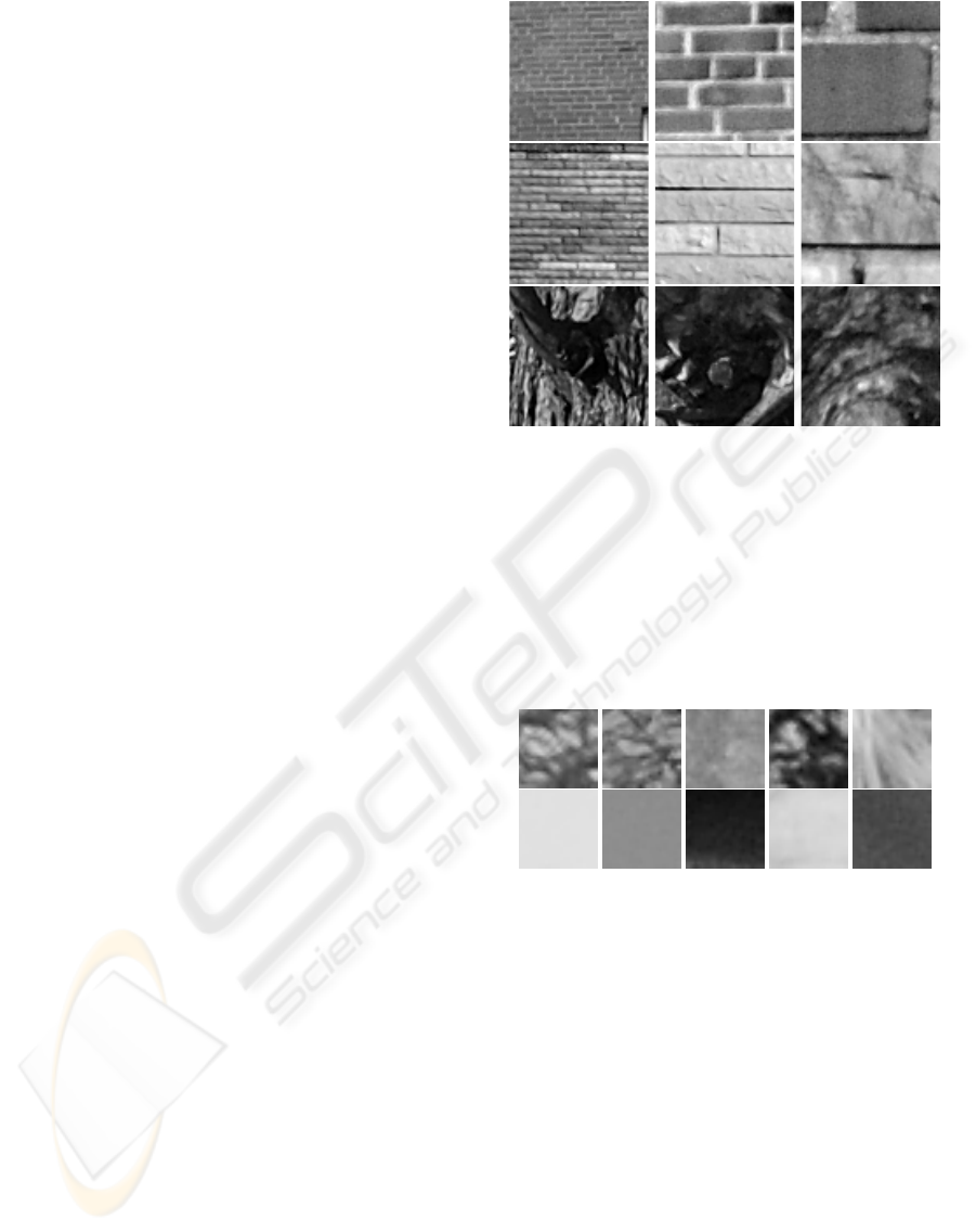
scales that can be seen in the 80×80 extracted patches
shown in figure 2. For example, in the most zoomed
image a brick is almost covering the whole 80 × 80
patch, while in the least zoomed image a large part of
the brick wall is contained in the patch. (The 80 × 80
patches are only shown for visualization of the con-
tents differences, while the complete regions are used
in the experiments.)
4 SINGULAR VALUE
DISTRIBUTION IN NATURAL
IMAGES
The proposed method depends on the distribution of
singular values in natural image patches. The distri-
bution of principal component and independent com-
ponents in natural images has received a lot of atten-
tion for some years, partly because its relation to the
front-end vision (Van Hateren and vad der Schaaff,
1998).
To analyze the distribution of singular values in natu-
ral image patches, 1000 randomly selected 25 × 25
patches from each image in the DIKU Multi-Scale
image database have been selected - approximately
800000 patches - and the corresponding singular val-
ues have been computed.
The first, not so surprising, conclusion is that patches
in natural images almost always have full rank - i.e.
the singular values are almost always strictly larger
than 0.
The distribution of singular values σ
1
and σ
2
are
shown in figure 4. The variance for the distribution of
σ
1
is large, and it is interesting that many patches have
values close to 25. The distribution for σ
2
is peaked
at zero but also have ’heavy tails’ - values relatively
far from zero. This is also the case for σ
i
where i > 2.
Figure 2: 80×80 patches extracted from the three sequence
shown in figure 1 at 3 different scales (index 1, 6 and 15).
The patches show the contents different at the different cap-
ture scales.
In figure 3 the patches with the largest σ
25
(top)
and smallest σ
25
(bottom) in five different images
are shown. The contents difference in the different
patches are striking - the patches with the largest σ
25
all contain large variations, while the patches with the
lowest σ
25
contain no or very little visible variations.
Figure 3: Each column show the patch with the largest (top)
and smallest (bottom) σ
25
in the same image. The content
difference is striking and clearly indicate the importance for
the small singular values for characterize the image content.
The distribution of the small singular values are
peaked at zero, but also show some variation and
’heavy tails’. Visual comparison of patches with high
and low σ
25
clearly indicates a content difference,
which implies that singular value reconstruction in-
dex is suitable for measuring image content.
5 EXPERIMENTS
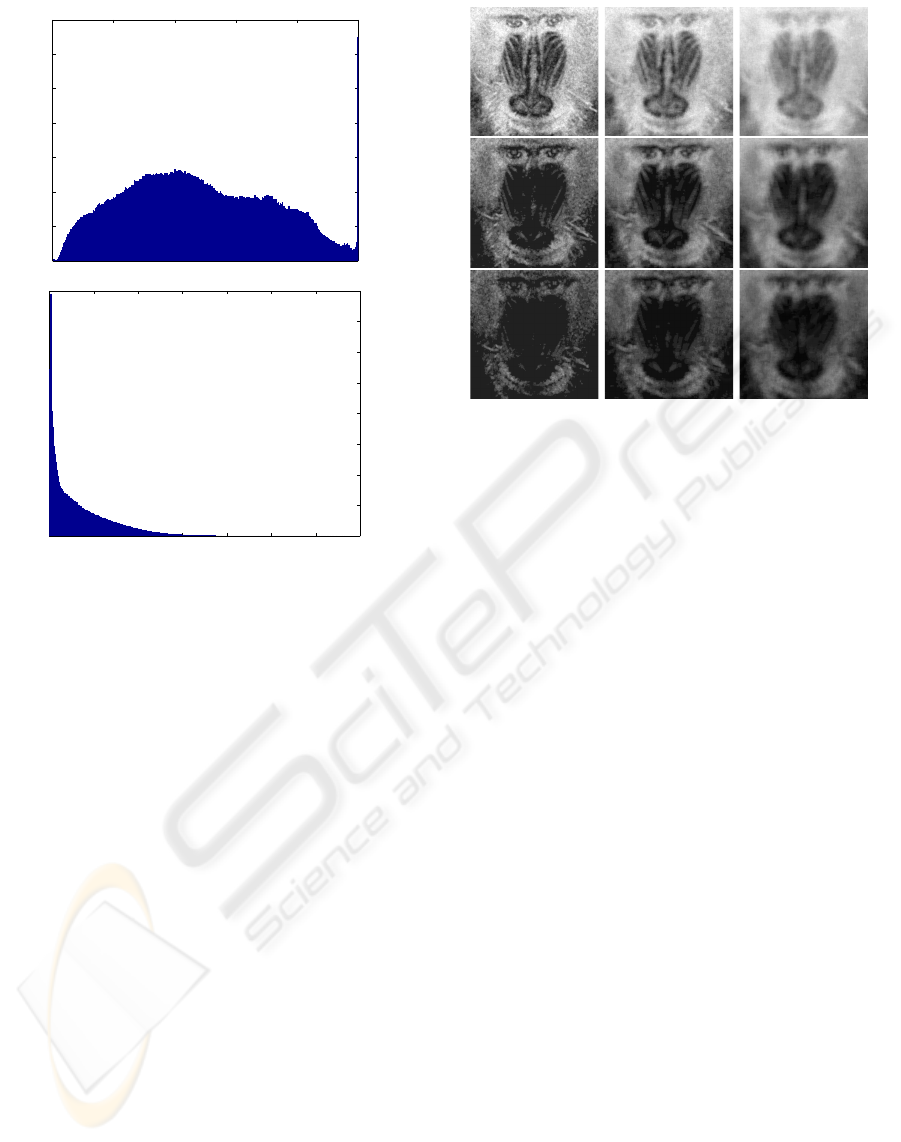
5.1 The Baboon Image
The baboon image is used only for demonstrating the
method. The baboon is a good test image because it
A SVD BASED IMAGE COMPLEXITY MEASURE
37

0 5 10 15 20 25
0
0.002
0.004
0.006
0.008
0.01
0.012
0.014
Distribution σ
1
0 1 2 3 4 5 6 7
0
0.01
0.02
0.03
0.04
0.05
0.06
0.07
0.08
Distribution σ
2
Figure 4: The distribution of singular values σ
1
and σ
2
for
natural images patches of size 25× 25. The variance for the
distribution of σ
1
is large (as expected), the distributions for
σ
2
is peaked at zero but also have ’heavy-tails’.
contains both very complex texture and large regions
with geometric structures. In figure 5 the spatial dis-
tribution of complexity is shown using different patch
sizes and error levels. White regions indicating high
complexity and black indicating low complexity. The
highly stochastic texture returns high complexity val-
ues at all scales and error levels, while the geomet-
ric structures return low complexity. As the patch
size grows larger the spatial distribution of complex-
ity gets smoother.
5.2 DIKU Multi-Scale Image Database
The image complexity measure is computed over the
different capture scales using different patch sizes and
error levels. The results are shown in figure 6.
The plot to the left and right, in figure 6, has the same
error level 0.35, but different patch sizes, 15 respec-
tive 25 pixels. Still the shape of the curves are very
similar. On the other hand the plot in the middle and
to the right have same patch sizes - 25 pixels -, but
different error level - 0.05 and 0.35 - and the curves
are very different which indicate that the error level is
more important than the patch size.
For sequence 02 the complexity at error level 0.05
first decreases roughly for the first 7 capture scales,
Figure 5: Patch based complexity measure of the baboon
image. Different patch size are used in the colon, from left
to right, the sizes are 9,15 and 25 pixels, and different re-
construction errors are used in the rows, from top to bottom,
0.1, 0.3, and 0.5.
and then increases for the last 7 capture scales. For
sequence 08 the complexity at error level 0.05 de-
crease quite rapidly at the first scales and then de-
creases slower for the remaining capture scales. For
sequence 05 the complexity decreases with increasing
capture scale.
The average number of singular values required for an
approximation at a fixed error level varies a lot over
the different capture scale. This indicate that the con-
tents in terms of complexity, change over the capture
scales which is clearly visiable from figure 2.
6 CONCLUSIONS
A patch based image complexity measure based on
the number of singular values that are required to ap-
proximate a patch at a given error level is presented.
The number of singular values is used to character-
ize the image content in terms of geometric structures
and texture.
The proposed method is motivated by the optimal
rank-k property of the truncated singular value ap-
proximation. The distribution of singular values in
patches from natural images seems to be peaked at
zero and have ’heavy-tails’. The image content in
patches with relatively large smallest singular value
are very different from the patches with relatively
small smallest singular value.
VISAPP 2009 - International Conference on Computer Vision Theory and Applications
38

0 5 10 15
5
6
7
8
9
10
11
12
Captured Scale
Image Complexity
seq 02
seq 05
seq 08
0 5 10 15
2
3
4
5
6
7
8
9
10
Captured Scale
Image Complexity
seq 02
seq 05
seq 08
0 5 10 15
10
11
12
13
14
15
16
17
18
19
20
Captured Scale
Image Complexity
seq 02
seq 05
seq 08
Figure 6: Complexity measure (y-axis)computed over different capture scales (x-axis) using different patch sizes and error
levels. From left to right: patch size 15 and σ
err
= 0.05, patch size 25 and σ
err
= 0.35, and patch size 15 and σ
err
= 0.05.
ACKNOWLEDGEMENTS
This research was funded by the EU Marie Curie Re-
search Training Network VISIONTRAIN MRTN-CT-
2004- 005439 and the Danish Natural Science Re-
search Council project Natural Image Sequence Anal-
ysis (NISA) 272-05-0256. The authors wants to thank
prof. Christoph Schn¨orr (Heidelberg University) and
PhD. Niels-Christian Overgaard (Lund University)
for sharing their knowledge.
REFERENCES
Buades, A., Coll, B., and Morel, J.-M. (2008). Nonlocal
image and movie denoising. IJCV, 76(2):123–139.
Chan, T. F. and Shen, J. (2005). Variational image inpaint-
ing. Communications on Pure and Applied Mathemat-
ics, 58.
Criminisi, A., P´erez, P., and Toyama, K. (2004). Region
filling and object removal by exemplar-based image
inpainting. IEEE IP, 13(9):1200–1212.
Cuzol, A., Pedersen, K. S., and Nielsen, M. (2008). Field
of particle filters for image inpainting. JMIV, 31(2-
3):147–156.
Efros, A. A. and Leung, T. K. (1999). Texture synthesis by
non-parametric sampling. In ICCV, pages 1033–1038.
Golub, G. H. and Loan, C. F. V. (1996). Matrix Computa-
tions. Johns Hopkins, 3rd edition.
Gustavsson, D., Pedersen, K. S., and Nielsen, M. (2007).
Image inpainting by cooling and heating. In SCIA 07,
pages 591–600.
Gustavsson, D., Pedersen, K. S., and Nielsen, M. (2009). A
multi-scale study of the distribution of geometry and
texture in natural images. In Preparation.
Hyv¨arinen, A. (1999). Survey on independent component
analysis. Neural Computing Surveys, 2:94–128.
Kass, M., Witkin, A., and Terzopoulos, D. (1988). Snakes:
Active contour models. IJCV, (4):321–331.
Kirby, M. (2000). Geometric Data Analysis. John Wiley &
Sons, Inc., New York, NY, USA.
Mumford, D. and Shah, J. (1985). Boundary detection by
minimizing functionals. In CVPT, pages 22–26.
Olsen, O. F. and Nielsen, M. (1997). Multi-scale gradi-
ent magnitude watershed segmentation. In ICIAP 97,
pages 6–13.
Randen, T. and Husoy, J. H. (1999). Filtering for tex-
ture classification: A comparative study. IEEE PAMI,
21(4):291–310.
Rudin, L. I., Osher, S., and Fatemi, E. (1992). Nonlinear
total variation based noise removal algorithms. Phys.
D, 60(1-4):259–268.
Sethian, J. A. (1999). Level Set Methods and Fast Marching
Methods. Cambridge University Press.
van Hateren, J. H. and vad der Schaaff, A. (1998). Inde-
pendent component filters of natural images compared
with simple cells in primary visual cortex. Proc. Royal
Soc. Lond. B, 265:359–366.
Weickert, J. (1998). Anisotropic Diffusion in Image Pro-
cessing. ECMI. Teubner-Verlag.
A SVD BASED IMAGE COMPLEXITY MEASURE
39