A METHOD FOR 3D MORPHING USING SLICES

Shamima Yasmin and Abdullah Zawawi Talib

School of Computer Sciences, Universiti Sains Malaysia, 11800 USM, Penang, Malaysia

Keywords: Morphing, Oriented Bounding Box (OBB), Alignment, Boundary Interpolation, Surface Reconstruction.

Abstract: 3-D morphing, in its simplest definition, is shape transformation between a pair of objects i.e. source and

target, by gradual, continuous and simultaneous dissolvement of the shape of source object to its target and

vice versa resulting in a number of intermediate shapes. Many algorithms have been developed for this

purpose with each one having its own speciality. In this paper, a novel algorithm is presented which is based

on slices. The technique originates from the concept of reducing a 3-D object to a number of slices in 2D

plane. In the algorithm, all of the 2D slices may not be oriented in either x, y, z or in a particular direction.

Orientation and rotation of the slices within a single body can be varied from one slice to another based on

the alignment of the object. Oriented Bounding Box (OBB) is used to determine the orientation of the

object. The advantages of the proposed method i.e. minimal user input, flexibility, dynamism and ease of

implementing over other 3D morphing algorithms are also discussed.

1 INTRODUCTION

Starting from the late eighties until the end of

nineties numerous algorithms on 3D morphing have

been developed. Now morphing has become an

indispensable tool in 3D animation industry. Not just

for the purpose of transforming from one shape to

another, morphing is also useful in incorporating

characteristics of different bodies in different

proportions to the morphed output.

In this paper a morphing algorithm which takes

into account of orientation and distortion of the

object is presented. Object is cut into slices along its

alignment. Oriented Bounding Box (OBB) is used to

determine the initial alignment of the object. The

more dense the slices, the more accurate is the

alignment (though there is an optimal limit on how

dense the slices could be). For all kind of objects,

this method works with minimal user input. The

simplicity, accuracy, versatility, flexibility and

extendibility of the algorithm meet all the criteria of

a good and efficient morphing algorithm based on

our survey on a number of morphing algorithms.

2 BACKGROUND

Depending on the various approaches, existing

morphing algorithms can be classified into the

following categories: a) Surface-based morphing:

consists of continuous mapping of small pieces of

polygonal surfaces of source object to those of target

object; b) Volume-based morphing: modifies voxel

values of a volume data set for smooth transition

between source and target shapes.

Surface-based approach uses user-defined

control fields such as point fields, line fields etc.

during morphing to map key features of source and

target objects ((Hong, 1988), (Parent, 1992),

(Lazarous, 1994), (Turk, 1999), (Lee, 1999)).

Surface-based methods are important because of its

ability to morph between objects of different types

of genus, but these methods also require a significant

amount of user input. Another troubling feature of

surface-based method is the problem of self-

intersection. It cannot guarantee that polygonal

surfaces will not pass through themselves, creating

self-intersecting intermediate result as found in

(Hong, 88).

Volume-based approach alleviates some of the

problems mentioned above. Among them, the

simplest approach is the cross-dissolving method

(Hughes, 1992) which at first transforms volume

data from spatial domain to frequency domain by

Fourier transform, then linearly interpolates volume

in frequency domain and again transforms back to

spatial domain. To enhance the smoothness of the

in-between volumes, Fourier transform has been

used by gradually removing high frequencies of

292

Yasmin S. and Talib A. (2009).

A METHOD FOR 3D MORPHING USING SLICES.

In Proceedings of the Fourth International Conference on Computer Graphics Theory and Applications, pages 292-301

DOI: 10.5220/0001786602920301

 SciTePress

source model, interpolating over to the low

frequencies of the second model and smoothly

adding in the high frequencies of the second model.

But Fourier transform does not localize in spatial

domain. In order to have a smooth transition, voxel

values of the entire volume are modified according

to the distance of the nearest iso-surface. This

problem can be solved by Wavelet transformation

(He, 1994), which localizes both in frequency and

spatial domain resulting in a multi-resolution fashion

so that high frequency distortion can be adjusted at

the desired level.

Both of the above mentioned methods have

difficulties in specifying slightly complex geometric

transformations such as object rotation. By relying

on the frequency information, the methods would

also have difficulties while associating with some

scalars such as colors, opacities and texture. This

problem can be alleviated by applying warping

before interpolation as found in (Lerois, 1995). Here

user-defined warp is applied on source and target

objects to resemble each other. Warped source

object and target object are then interpolated.

Instead of using point and line control fields in

3-D volume morphing, user-specified disk field

(Chen, 1996) can be used. Equal number of disks are

applied on both source and target to establish

correspondence between them. Each disk has its

own normal direction which helps in considering

distortion of the body.

Payne et al. introduces ‘Distance Volume’ mea -

sured by computing the shortest distance of each

voxel within the volume to the surface of the object.

Distance field is transformed to a function to meet

greater, equal or lesser “blobbiness” between the

source and target objects. Once the distance field for

the input surfaces are computed, interpolation is

performed in between the surfaces.

In (Breen, 2001), the way in which points on the

surface moves is used to establish connection

between source and target. Every point on the source

surface moves in the direction of the normal at that

point with a velocity proportional to the signed

distance at that point in 3-D space from target

surface and vice-versa. Those parts of source which

are outside the target contract whereas inside parts

move in the direction of surface normals and

expand.

Shape transformation using implicit function

(Turk, 1999) is constructed by reducing a 3-D

volume to a stack of 2-D slices along any of the

major axes. Implicit functions of each pair of 2-D

slices are determined using a set of constraints i.e.

location, weight, scalar values etc. The resultant 2-D

contour is established by interpolating each pair of

implicit functions and this is repeated for each pair

of slices between source and target objects along the

third axis.

From the above discussion, it is obvious that

volume-based approach has got some advantages

over surface-based approach though each approach

has its own advantages. It is imperative that we

strive to develop a new volume-based morphing

algorithm which optimizes user input, considers

rotation/orientation of rigid body during morphing

and preserves smooth transition between source and

target.

3 ALGORITHM OVERVIEW

The algorithm mainly consists of the following

major steps :

 Data Traversal and Slicing of Data;

 Boundary Extraction;

 Boundary Projection and Boundary Interpo-

lation;

 Orientation and Translation of Boundaries;

 Surface Reconstruction.

3.1 Data Traversal and Slicing of Data

Source and target data are collected. The initial

orientation along which the data are subdivided in

the first step of the binary subdivision is defined

along any of the directions of the Oriented Bounding

Box (OBB) (Gottschalk, 1996). An Oriented

Bounding Box (OBB) is a bounding box that does

not necessarily align itself along the coordinate axes.

OBB is constructed from the mean and covariance

matrix of the cells and their vertices that define the

dataset. The eigen vectors of the covariance matrix

are extracted, giving a set of three orthogonal

vectors that define the alignment of the dataset.

Figure 1 shows the difference between a normal

bounding box and an oriented bounding box. No

doubt, an oriented bounding box more closely fits

the data than a normal bounding box. The purpose of

choosing the oriented bounding box is to allow

checking of the longitudinal direction of dataset

from its oriented bounding box rather than from

normal bounding box. The OBB only bounds the

“geometry” attached to the cells if the convex hull of

the cells bounds the geometry. This is done in order

A METHOD FOR 3D MORPHING USING SLICES

293

to negate the effects of the extreme distribution of

the points.

Figure 1: (a) Normal Bounding Box and (b) Oriented

Bounding Box.

Eigen vectors describe the maximum, medium

and minimum variance of concentration of point

clouds. Usually either maximum or medium direc -

tion of the eigen vectors are used as the direction of

the initial alignment. The ‘maximum’ direction

shows the maximum amount of concentration of the

cells of the data along that direction, whereas the

‘medium’ direction exhibits less amount of concen -

tration than maximum direction and the ‘minimum’

direction shows the least amount of concentration or

the least alignment of the cells along that direction.

The first subdivision takes place along a plane

centered at the center of the Oriented Bounding Box

(OBB) of the object with normal along the initial

alignment. This step, called ‘step 0’, divides the data

into two end parts. In each of the subsequent steps,

the number of slices is doubled.

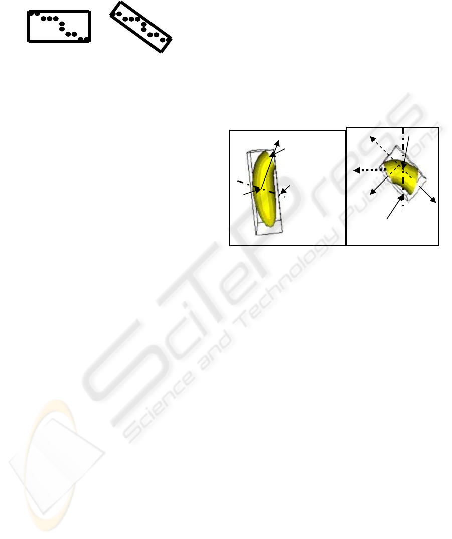
In the next step i.e. ‘step 1’, each of the two end

pieces found from ‘step 0’ is wrapped with OBB and

tested whether the longitudinal direction of the

alignment of the sliced end is still within the

maximum or medium direction of the OBB. If the

alignment is still within maximum/ medium

direction, a line joining the center of the previous cut

plane and the center of the OBB is used as the

direction of the cut plane normal for the ends in that

step (Figure 2). Otherwise ends are sliced along the

cut plane normal found in the previous step which is

used for any further subdivision of the ends and in

the subsequent steps no further checking on the

alignment is done. At the end of ‘step 1’, the data is

divided into four parts i.e. two end parts and two

middle parts.

Before further subdivision of the ends, if

necessary, checking is done for the alignment of the

two sliced ends. The procedure described in ‘step 1’

is followed for further subdivision of the two ends.

For the middle parts, data is sliced along the plane

with center as the center of the OBB and normal

directed along the resultant normals of the two ends

of the middle data (Figure 2(a)). Slicing is continued

along the longitudinal direction until the desired

number of steps is reached. In each subsequent step,

the number of slices is doubled at each step. The

default longitudinal direction is the ‘maximum’

direction of the eigen vectors and the default number

of steps for binary subdivision of the data is ‘four’.

To provide more flexibility, the initial longitudinal

direction as well as the number of steps can be

defined by the user. We indicate the maximum

alignment as ‘0’, the medium alignment as ‘1’ and

the minimum as ‘2’. Therefore, the users are allowed

to vary the morphed output based on the initial

alignment. Subdivision can also be forced to happen

along any particular direction or along any of the

axes i.e. x, y or z to generate parallel slices.

(a) (b)

C2 =

N1= Line joining C1 and O1

Center

OBB

Figure 2: Division of (a) the End Data and (b) the Middle

Data.

The steps involved in slicing a given data with

default initial settings are depicted in Figure 3. After

reaching the desired number of steps, cut edges of

the ends are usually still a bit far from the tip. In

order to extract a proper outline of the object, ends

near the tip need to be extracted. For this purpose,

two ends are traversed along the tip. Usually no fur -

ther checking for the alignments of the two ends are

needed now as the current alignments of the sliced

ends are usually not along the maximum or the

medium direction of the OBB of the two sliced

ends. So for any further subdivision, the normal is

usually along the direction which was found at the

step before the last checking step and traversing

towards the tip is continued along that direction until

it is close enough to the tip. Now the ends are again

divided into two parts. At this stage, each of the two

end slices which were found at the end of the last

step consists of two end parts with very thin top ends

near the tips as shown at the bottom of Figure 3.

N =N2 + N3’

N3’

O1 = Center o

Previous Cut Plane

Next cut plane is along normal

N with Center C2.

(b)

C1=

Center

OBB

Next cut plane is

along Normal N1

with Center C1.

(Alignment is with

-in maximum/ medi-

um)

(a)

GRAPP 2009 - International Conference on Computer Graphics Theory and Applications

294

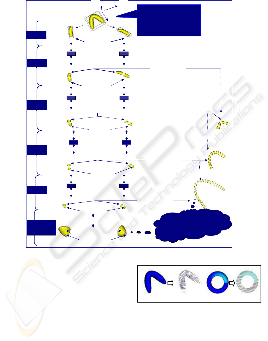
Figure 3: Traversal and Slicing of a Given Data.

3.2 Boundary Extraction

Only boundaries of the slices are extracted (Figure

4). As discussed above, in ‘step 0’, data is divided

into two parts. In each of the subsequent steps, the

number of slices are doubled. Hence in ‘step 4’,

there are 2

(4+1)

i.e. 32 slices. From 32 slices 31

boundaries can be extracted. Then boundaries at the

ends which are determined after the specified

number of steps is reached are also added. Two such

boundaries at the two ends result in a total of 33

boundaries each. Hence in ‘step 4’, the number of

extracted boundaries (for each source and target) is

computed as follows:

(step+1)

+ 1 = 2

(4+1)

+ 1= 2

+ 1 = 33

Figure 4: Extraction of Source and Target Boundaries.

3.3 Boundary Projection and

Boundary Interpolation

Both source and target boundaries are projected onto

the XZ plane and centered at the origin. Each of the

source and target boundaries are traversed along the

direction of their minimum X (X

min

) to maximum X

Initial Conditions:

1.No. of Step = 4 (default);

2. Alignment = 0 (default)

(maximum = 0, medium = 1,

minimum = 2)

2 0

2 End Parts

Alig

nment

on o

Yes

Alig

nment

on o

Yes

Alig

nment

Division of the Ends

Yes

Alig

nment

Division of the Ends

Yes

Step 4

Alig

nment

on o

Alig

nment

Division of the Ends

2EndParts

2 Thin End Parts Parts

Alig

nment

Division of the Ends

Yes

Alig

nment

Division of the Ends

Yes

2 End Parts

30 Middle Parts

14 Middle Parts

Determination

of Top Ends

Division of the Middle Parts

Traversal alon

the Ti

2Thicker Middle Parts

2 End Parts

6 Middle Parts

Division of the Middle Parts

2 Middle Parts

Step 3

Step 2

Step 1

Step 0

At the end of data traversal,

data is divided into 2 end

arts and 32 middle

arts.

Target Boundaries

Source Boundaries

A METHOD FOR 3D MORPHING USING SLICES

295

max

) with a traversal plane defined as (1,0,0). For

each source and target boundaries, traversal spacings

are determined separately. Equal number of

traversals is performed for both source and target

data. Traversal spacing is determined as follows:

Spacing = (X

max

– X

min

)/ Number of Traversals

Source and target boundary points are extracted

from the traversals. If the number of extracted points

in any cut plane happens to be odd, it is made to be

even. Next interpolation is performed onto the XZ

plane. For simplicity linear interpolation is used in

our implementation. Here it should be noted that

only one normal is extracted per boundary regardless

of whether any particular boundary consists of

multiple holes or empty spaces. Also each boundary

has one center irrespective of the irregular geometric

configuration of that particular boundary.

Three special cases need to be considered during

interpolation. They are as follows:

Case 1: Both Source and Target Boundaries

Contain no Empty Spaces.

Source points are just

interpolated with target points. Enhancement of the

interpolation process can be carried out when both

source and target have equal number of regions and

there are more than one region in both. Region is an

area where the number of points extracted by the cut

plane is the same while traversing along the X axis.

In Figure 5, both source and target boundaries

consist of equal number of regions i.e. 3 (two 2-

point region and one 4-point region). Hence the

interpolated point clouds also have three regions.

Case 2: Only One of the Source and Target

Boundaries Contains Empty Spaces. The number

of empty spaces is calculated for the boundary

which contains empty spaces. Then equal number of

empty spaces are inserted into the other boundary so

that empty space will appear in the interpolated

point clouds.

Case 3: Both Source and Target Boundaries

Contain Empty Space. When there are equal

number of empty spaces in both source and target

boundaries, we have equal number of regions. Thus

corresponding regions from both source and target

can be interpolated. However when there are

unequal number of empty spaces/ regions, rightward

and leftward traversals are carried out until either

one of source or target is exhausted (Figure 6).

Corresponding regions during the traver -sal are just

mapped and interpolated while the remaining

regions can just be mapped if the exhausted side

ends with an empty space. Otherwise a process

similar to Case 2 above is applied by inserting into

the region of the exhausted side the same number of

empty spaces left in the non-exhausted side.

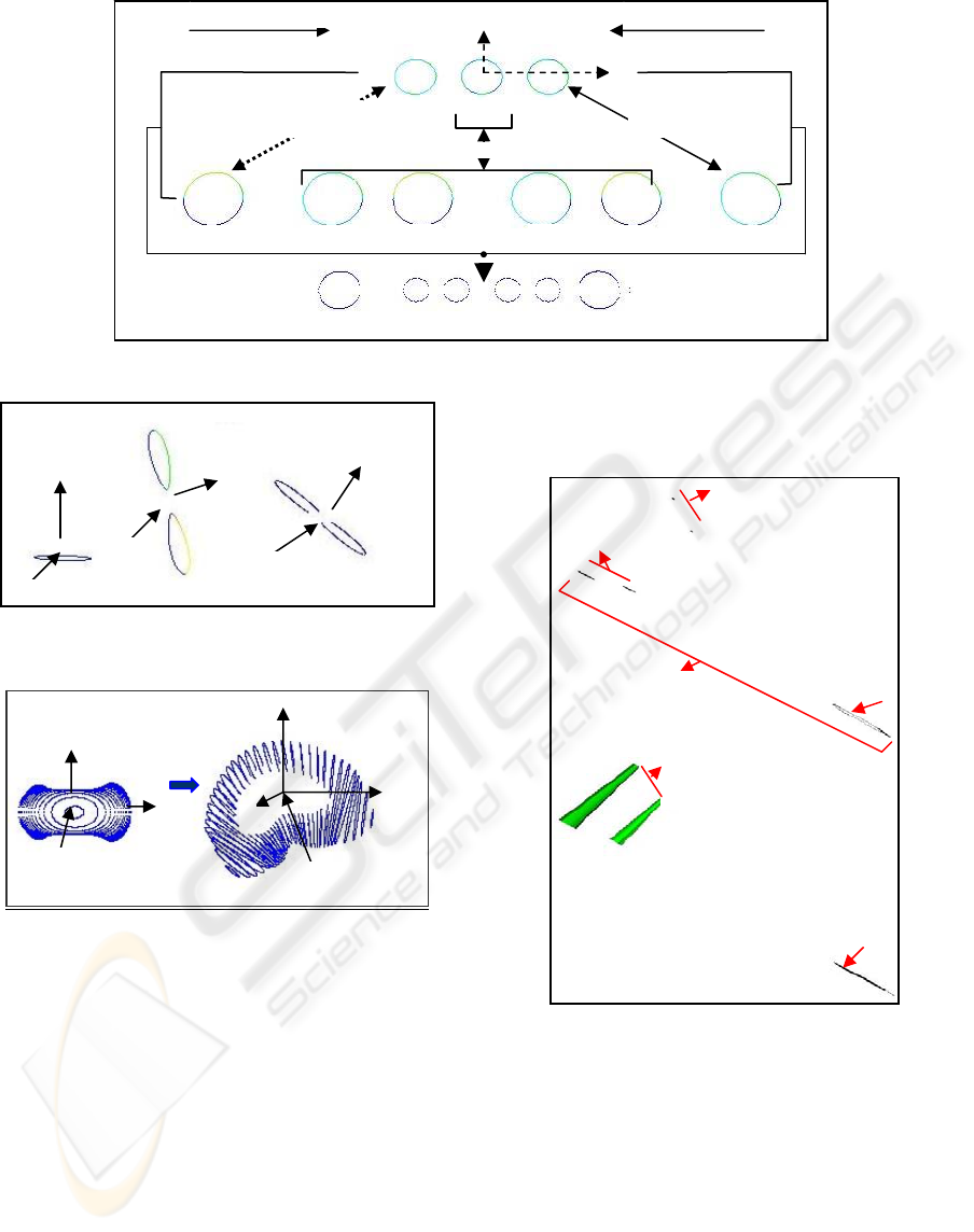
Figure 5: Interpolation of Points after Region Separation.

3.4 Orientation and Translation of

Interpolated Boundaries

Each of the interpolated boundary already projected

onto the XZ plane is oriented along the resultant

normal of each of the source and target boundaries

and translated to the average center of each of source

and target boundaries (Figure 7). When all the

interpolated boundaries are oriented as well as

translated, we get the outline of the morphed output.

Figure 8 describes this sequence.

3.5 Surface Reconstruction

From the stack of oriented and translated bounda -

ries, surface of the morphed object is constructed.

Each of the boundaries merges with the next boun-

dary by dividing the in-between space of the two

consecutive boundaries into a number of cells and

each cell is connected to its neighboring cells. Sur -

face construction is performed by only considering

each of the two consecutive boundaries.

2-pt Region (At an

particular distance

along X, number o

intersected points

by a plane (1,0,0), is

Interpolated Point Clouds

(

)

(0,0,0)

4-point Region (At any particular distance along X,

number of intersected points by a plane (1,0,0), is 4).

SOURCE TARGET

(

)

2-point

ion

4-point

Region

2-point

Region

GRAPP 2009 - International Conference on Computer Graphics Theory and Applications

296

Rightward Traversal Leftward Traversal

Figure 6: Interpolation case when there are unequal number of empty spaces between source and target.

Figure 7: Orientation and Translation of a Single

Interpolated Boundary.

Figure 8: Orientation and Translation of All Interpolated

Boundaries.

This simplifies the overall surface reconstruction

process as where data is highly irregular, necessary

modification among cell coordinates is limited to

only two consecutive boundaries. Surface

reconstruction in detail is discussed next.

3.5.1 Separating Disconnected Region

Each consecutive boundary may have regions which

are disconnected from one another (Figure 9(a)).

Nearest neighbor searching is carried out to find this

kind of regions. The disconnected regions are

horizontally mapped (for better effect) and the other

regions are to be vertically mapped (Figure 9(b)).

The details of the vertical mapping are discussed

in the next sub section.

Figure 9: Separating Disconnecting Regions between Two

Consecutive Boundaries.

3.5.2 Basic Cell Construction

After region separation, two consecutive point/ cell

arrays (representing two consecutive slices) are

obtained and vertically mapped. The two arrays

which contain the number of interpolated points at

each index need to be compressed so that the process

of mapping can be carried out in an easier and

straightforward manner.

Point clouds in top slice

with only one region

Point clouds in bottom slice

with two separate regions

ion 1

Region 2

After region separation point clouds in

top slice vertically mapped with region 1

of bottom slice

Disconnected region 2

in bottom slice is

horizontally mapped

(a)

(b)

(0,0,0)

N = (N1 + N2)/2

C = (C1 + C2)/2

Source Slice

Tar

et Slice

Oriented and Inter

olated Slice

ion1

ion1 Re

ion3Re

ion2

ion4

ion5 Re

ion6

ion3

Region 1 of Source maps

with Re

ion 1 of Tar

Region 3 of Source maps

with Re

ion 6 of Tar

ion 2 of Source ma

s with Re

ion 2 …. Re

ion 5 of Tar

Interpolated Points

(c)

A METHOD FOR 3D MORPHING USING SLICES

297

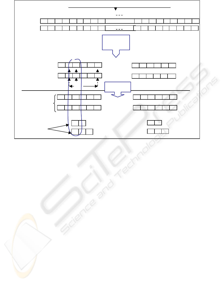
Two Arrays Containing the Number of Interpolated Points

0 1 2 3 4 5 6 7 8 9 40 41 42 43 44 45 46 47 48 49

Index No:

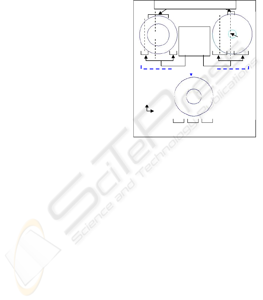
Figure 10: Basic Cell Construction between Two Consecutive Interpolated Boundaries.

Figure 10 shows the process of compressing two

consecutive arrays. In the compression, the arrays

are transformed into two new arrays each: region

number array (where region numbers are stored) and

number of occurrences array (where the number of

occurrences of each region number are stored).

Firstly, the size of both arrays should be made equal

using a heuristic approach. Sometimes some index

values are dissolved and some are omitted in order

to make the size of both arrays equal. Corresponding

values of the number of occurrences arrays should

also be made equal so that they are ready to be

vertically mapped. In the case of unequal values, the

larger of the two values is made equal to the smaller

number by removing excess number of that

particular number of occurrences value.

Corresponding numbers in the two region number

arrays should also be equal for the purpose of

vertical mapping. If they are not equal, a further

processing needs to be done. The process starts with

finding the nearest matched index values of the

region number arrays by traversing to the left and

the right. The nearest matched values will ensure

better continuity between different-numbered

regions. Next the corresponding region numbers are

split into two portions where the values of the region

number of the first portion is derived from the

continuous mapping of the nearest matched index

values to the corresponding region number values

and the values of the region number of the second

portion are the remaining region numbers resulting

from the split.

In the example (Figure 10), the first

discrepancy occurs at index number ‘2’ and the

nearest matched values are at index number ‘1’ with

a value of ‘4’ and ‘4’. The current values (i.e. 8 and

6) need to be split into two portions. The first

portions are made equal to ‘4’ and the second

portions are assigned the remaining values (8-4 = 4

and 6-4 = 2).

At the end of the entire processing, two

sets of region number arrays are obtained. The top

set (Figure 10(a)) now consists of equal region

number and can therefore be vertically mapped

whereas each of the bottom set (Figure 10(b)) is to

be horizontally mapped separately. Enhancement is

carried out in surface reconstruction when empty

space is met or at the transition point between two

different-numbered regions.

Number Array

Index No:

Array

Each Array is

Compressed

2 Arrays

4 2

2 4 2

At the End of the

Entire Processing

---

4 6

Number of Occurrences Array

Region Number Array

0 1 2 3 4 5

Vertical Mapping

between

Corresponding Cells

Separate

Horizontal

Mapping

(

)

(

)

GRAPP 2009 - International Conference on Computer Graphics Theory and Applications

298

4 IMPLEMENTATION AND

RESULTS

The algorithm has been implemented using C++

with Visualization Tool Kit (VTK) as graphics plat -

form. In Figure 11(a), a sequence of three interme-

diate stages is generated using ‘5’ as the number of

steps with the initial direction of traversal for source

as well as target along the maximum direction of the

eigen vector i.e. ‘alignment = 0’. Using ‘4’ as the

number of steps, the same sequence is generated

without producing major distortion to the eye. As the

number of step increases, the number of slices is

doubled which also increases the overall run time.

Figure 11(b) shows the morphing sequence

between two tori each with different radius with the

initial direction of traversal along the minimum

direction of eigen vector i.e. ‘alignment = 2’ for both

source and target. In Figure 11(c), a morphing

sequence between a complex object and a bent pipe

has been generated. Here the initial direction of

traversal for the source is along the minimum direc-

tion of eigen vector i.e. ‘alignment = 2’ whereas the

initial direction of traversal for the target is along the

maximum direction of eigen vector i.e. ‘alignment =

0’. Figure 11(d) shows the morphing sequence

between a conic spiral and a torus with the initial

directions of traversal for both source and target

along the maximum direction of eigen vector i.e.

‘alignment = 0’.

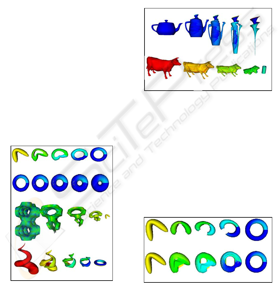
Figure 11: Morphing Sequence between Source (left most)

and Target (right most) for Different Eigen Vectors as

Initial Direction of Traversal.

As highlighted in Section 3.1, the initial direction

of traversal can also be forced to happen along the

principal axis. In Figure 12(a), morphing sequence

between a teapot and a parametric surface ‘dini’ has

been generated. Here the initial directions of

traversal for both source and target are along the Y-

axis. Figure 12(b) shows the morphing sequence

between a cow and a cylindrical object. Here the

initial direction of traversal for the source is along

the X-axis and the initial direction of traversal for

the target is along the Y-axis.

(a)

(

)

Figure 12: Morphing Sequence between Source (left most)

and Target (right most) for Different Principal Axis as

Initial Direction of Traversal.

Figure 13 compares the gradual morphing

sequence between the same source and target as

used in Figure 11(a) when initial direction of tra -

versal for source/ target changes. Figure 13(a) shows

the gradual transformation between source and

target when the initial directions of traversal for

source and target are along medium and maximum

direction of the eigen vector i.e. ‘alignment = 1’ and

‘alignment = 0’ respectively. Figure 13(b) shows the

morphing sequence when the initial directions of

traversal for both source and target are along the

minimum direction of eigen vector i.e. ‘alignment =

2’.

Figure 13: Morphing Sequence between the Same Source

(left most) and Target (right most) for Different Eigen

Vectors as Initial Direction of Traversal.

(a)

(

)

(

)

(

)

(

)

(

)

A METHOD FOR 3D MORPHING USING SLICES

299

Instead of principal axis, if morphing sequence is

generated along the longitudinal direc -tion, warping

in rigid body is also considered when it is needed.

Figure 14 compares this situation. In Figure 14(a),

the morphing sequence is generated with initial

direction of traversal along the principal axis X and

Y for source and target respectively whereas in

Figure 14(b), the morphing sequence is generated

with the initial direction of traversal for both source

and target along the maximum direction of eigen

vector i.e. ‘alignment = 0’.

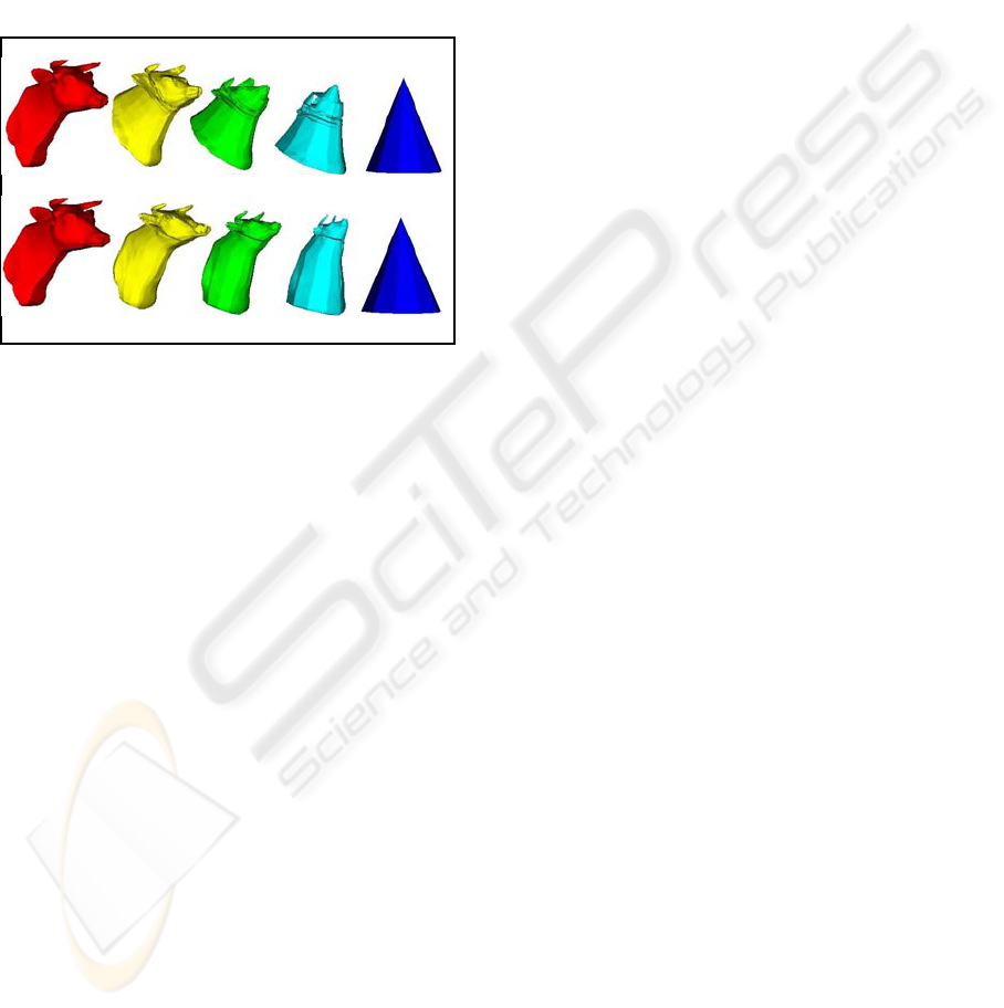
Figure 14: Morphing Sequence between the Same Source

(leftmost) and Target (rightmost) with (a) Principal Axis

and (b) Eigen Vector as Initial Direction of Traversal.

5 DISCUSSION

This section compares the proposed algorithm with

some other existing morphing algorithms on the

basis of a number of criteria for good morphing.

Most surface-based methods consider the

distortion/rotation of the rigid body, but division of

both source/ target into a number of morphing

patches or meshes is needed at the expense of a large

number of user input and longer pre-processing

stage ((Kent, -1992), (Lazarous, 1994), (Gregory,

1998), (Breen, 2001)). The proposed algorithm

works without any user input with default initial

settings (‘number of steps = 4’ and ‘alignment =

max’). If variations in the number of steps and

alignments are desired, the user just needs to specify

these two variables. The number of slices can also

be reduced by varying the number of steps. This

automated method of reducing the number of slices

as well as run time is absent in the most other

algorithms. In most other existing algorithms,

specific number of user-defined disk fields (Chen,

1996) or point/line fields ((Kent, 1992), (Lazarous,

1994), (Gregory, 1998), (Breen, 2001)) are used.

Varying these fields involves a considerable amount

of user intervention and longer pre-processing time:

minor variation in these fields can generate a major

variation in the output. The proposed algorithm

automatically traverses the data along its alignment

and is free from any inaccurate user intervention and

at the same time if needed allows user to specify the

initial direction of traversal.

Simplicity is one of the major characteristics of

the proposed algorithm. Some early surface-based

algorithm preserves this feature but at the same time

fails when the object is a bit complex producing self-

intersecting intermediate objects (Hong, 1988). In

the proposed algorithm, aligned slices are extracted

from data traversal and before interpolation, slices of

the corresponding source and target slices are

projected onto the XZ plane. Hence chances of self-

intersection are very slim as that can happen when

triangulated surfaces are interpolated or extracted

slices are not properly aligned.

(a)

Another important feature of a good morphing is

that intermediate outputs should be confined to the

geometric features of source and target only.

However sometimes unnecessary fea -tures are also

seen among the intermediate morphed objects

((Gregory, 1998), (Kent, 1992)). In the pro -posed

algorithm smooth transition takes place bet -ween

source and target. Orientation as well as rota -tion of

a rigid body are preserved while morphing .

(

)

Some volume-based methods use discrete

mathematical function in morphing between

complex objects ((Hughes, 92), (He, 1994), (Turk,

1999)) generating smooth output using sophisticated

interpolation technique. But interpolation is only one

facet of morphing. The major shortcoming of these

methods is that they overlook the curvature of rigid

body while morphing, which is one of the most

important properties needed to be considered for

morphing between curved objects. The proposed

algorithm nicely fills in the gap. Some volume-based

algorithms alleviate this problems ((Payne, 1992),

(Breen, 2001)). However they are highly sensitive to

the user-specified initial overlapping of source and

target. These methods have weakness around the

regions of high curvature: accuracy of intermediate

objects also depends on the accuracy of user-defined

overlapping of source and target. This sometimes

results in incomplete morphed output in case of

curved objects. The proposed algorithm shows more

consistency than these methods.

In the proposed algorithm, instead of traversing

along the longitudinal direction of data, traversal can

also take place along any particular direction

producing different morphing sequences. This

flexibility may be difficult to achieve in surface-

GRAPP 2009 - International Conference on Computer Graphics Theory and Applications

300

based algorithms or in some volume-based

algorithms which exhibit characteristics like surface-

based algorithms (Lerois, 1995). Some volume-

based algorithms can consider this but may involve

considerable user intervention ((Payne, 1992),

(Chen, 1996), (Breen, 2001)). Morphing involving

discrete mathematical functions for interpolation

((Hughes, 1992), (He, 1994), (Turk, 1999)) is

capable of traversing along only a specified

direction.

Now let us analyze the algorithm in terms of

efficiency. In field morphing, control data sets are

used to specify coordinate mapping hence time

complexity is usually Ө(nm) as all coordinates of a

single dataset are more or less influenced by all

control fields (Chen, 1995). Here ‘n’ is the size of

volume and ‘m’ is the number of control fields. In

the proposed method, control fields i.e. slices are

automatically determined during data traversal and

these control fields have little influence or control in

coordinate mapping: only coordinates of respective

boundaries are influenced. Hence if the number of

extracted coordinates from each boundary is ‘p’ and

the number of automatically defined slices (‘m’) are

considered as control fields, then time complexity is

Ө(mp + m). Here ‘mp’ can be equated with the

volume size ‘n’ hence time complexity for the

proposed algorithm is Ө(n + m) which is much less

than volume morphing using disk field Ө(nm)

(Chen, 1996).

6 CONCLUSIONS

Simplicity and flexibility are two major characteris -

tics of the proposed algorithm which have made it

more dynamic and extendible than other existing

morphing algorithms. Future work includes exten -

ding the algorithm in order to show the extendibility

of the method by incorporating influence shape

while morphing including multiple influences and

exploitation of the method in parallel/distributed

computing environment as simple data structure of

sliced body and binary subdivision is suitable for

both data as well as functional partitioning.

REFERENCES

Hong, T., Magnenat-Thalmann, N., Thalmann, D., 1988.

A General Algorithm for 3D Shape Interpolation in a

Facet-based Representation. In Proceedings on Gra -

phics Interface `88, pages 229-235.

Hughes, J., F., 1992. Scheduled Fourier Volume

Morphing, ACM SIGGRAPH Computer Graphics:

26(2): 43-46.

Payne, B., Toga, A., 1992. Distance Field Manipulation

of Surface Models , IEEE Computer Graphics and

Applications: 12(1), 65-71.

Kent, R., J., Carlson, W., E., Parent, R., E., 1992. Shape

Transformation for Polyhedral Objects, In Procee

dings of ACM SIGGRAPH’99, pages 335-342.

Kaul, A., Rossignac., J., 1992. Solid Interpolationg Defor -

mations: Construction and Animation of PIPS,

Computers and Graphics: 16(1), 107-115.

Lazarous, F., Lopes, Verroust, A., 1994. Feature based

Shape Transformation for Polyhedral Objects, In Fifth

Eurographics Workshop on Animation and

Simulation, pages 241-254.

He, T., Wang, S., Kauffman, A., 1994. Wavelet-based

Volume Morphing, In Proceedings of IEEE

Visualization, page 85-92.

Lerois, A., Garfinkle, C., D., Levoy, M., 1995. Feature-

based Volume Metamorphosis, Computer Geaphics

29, “Annual Conference Series”, pages 449-456.

Chen, M., Jones, M., W., Townsend, P. 1995. Methods for

Volume Morphosis, In Image Processing and

Broadcast for Video Production, Y. Parker and S.

Wilbur (eds), Springer-Verlag, Berlin, pages 280-292.

Chen, M., Jones, M., W., Townsend, P., 1996. Volume

Distortion and Morphing Using Disk Fields,

Computers and Graphics: 24(2), 567-575.

Gottschalk, S., Lin, M., C., Manocha, D., 1996. Obbtree:

A Hierarchical Structure for Rapid Interference

Detection, Computers and Graphics (30), “Annual

Conference Series”, pages 171-180.

Gregory, A., State, A., Lin, M., C., Manocha, D.,

LivingSton, M.,1998. Feature-based Surface Decom-

position for Correspondence and Morphing between

Polyhedra, In Computer Animation and Procee

dings’98, pages 64-71.

Lee, A., W., F., Dobkin, D., Sweldens, W., Schrőder, P.,

1999. Multiresolution Mesh Morphing, In Proceedings

of SIGGRAPH’99, pages 343-350.

Turk, G., O’Brien, J., F., 1999. Shape Transformation

using Variational Implicit Functions, In Proceedings

of ACM SIGGRAPH’99, pages 335-342.

Breen, D., E., Whitaker, R., T., 2001. A Level Set

Approach for the Metamorphosis of Solid Models,

IEEE Transactions on Visualization and Computer

Graphics: 7(2), 173-192.

A METHOD FOR 3D MORPHING USING SLICES

301