LIVER SEGMENTATION USING LEVEL SETS

AND GENETIC ALGORITHMS

Dário A. B. Oliveira, Raul Q. Feitosa

Department of Electric Engineering, Catholic University of Rio de Janeiro, Rio de Janeiro, Brasil

Mauro M. Correia

Unigranrio and National Cancer Institute-INCA, Rio de Janeiro, Brasil

Keywords: Medical Imaging, Liver Segmentation, Computer Tomography, Level Sets, Genetic Algorithms.

Abstract: This paper presents a method based on level sets to segment the liver using Computer Tomography (CT)

images. Initially, the liver boundary is manually set in one slice as an initial solution, and then the method

automatically segments the liver in all other slices, sequentially. In each step of iteration it fits a Gaussian

curve to the liver histogram to model the speed image in which the level sets propagates. The parameters of

our method were estimated using Genetic Algorithms (GA) and a database of reference segmentations. The

method was tested using 20 different exams and five different measures of performance, and the results

obtained confirm the potential of the method. The cases in which the method presented a poor performance

are also discussed in order to instigate further research.

1 INTRODUCTION

In medical imaging analysis, image-guided surgery

and organs visualization, segmentation is a crucial

step. This step is particularly arduous in abdominal

CT images because different organs lie within

overlaping intensity value ranges and are often near

to each other anatomically.

Numerous techniques have been proposed in the

literature for extraction of organs contours in

abdominal CT scans. They can be roughly divided in

two main groups: model driven and data driven

approaches.

Model driven techniques (e.g. Lamecker et al.,

2004) use pre-defined models to segment the desired

object from the available images. This kind of

technique basically searches the images for instances

that fit a given model described in terms of object

characteristics such as position, texture and spatial

relation to other objects.

Data driven techniques (e.g. Fujimoto et al.,

2001) try to emulate the human capacity to identify

objects using some similarity information present on

image data, automatically detecting and classifying

objects and features in images. Many of them use

known techniques such as region growing and

thresholding, combined with some prior knowledge

about the object being analised.

This paper proposes a model driven method

based on level sets to segment the liver with an

evolutionary approach to select its paremeters. Using

an initial user-defined liver segment in one slice, the

method segments the liver through all other slices. It

uses a Gaussian fit to define the speed image where

the level sets propagates. The initial solution at each

slice is defined as the region previously segmented

on an adjacent slice. Experiments using five exams

as training set and other 15 exams for validation

indicate the outcome of our method.

The subsequent text is organised in the following

way. Section 2 presents theorectical fundamentals of

level sets and genetic algorithms. Section 3 presents

the proposed segmentation method in details, section

4 presents the parameters estimation experiments,

section 5 reports some results, and the main

conclusions are presented in section 6.

154

A. B. Oliveira D., Q. Feitosa R. and M. Correia M. (2009).

LIVER SEGMENTATION USING LEVEL SETS AND GENETIC ALGORITHMS.

In Proceedings of the Fourth International Conference on Computer Vision Theory and Applications, pages 154-159

DOI: 10.5220/0001787401540159

 SciTePress

2 THEORETICAL

FUNDAMENTALS

In this section we introduce theoretical fundamentals

related to the level sets method and present then an

overall description of genetic algorithms.

2.1 Level Sets

Level set methods were developed by Sethian and

Osher (Osher and Sethian, 1998) and firstly

introduced in medical imaging by Malladi et al.

(Malladi et al, 1995).

Level set is a continuous deformable model

method with implicit representation. Its main idea is

to embed the deformable model in a d+1

dimensional space, to segment iteratively an object

in a d dimensional space, using partial differential

equations. The main advantage of level sets is that it

allows changes of surface topology implicitly. As it

embeds the evolving surface, also called interface, in

a higher dimensional function, this interface can

split into several connected components or merge

from different connected components naturally, and

the embedding level sets function remains

continuous.

Considering ψ(x,t) the level sets function, x the

position vector and t the time step of the level set

evolution, the evolving surface is represented as the

zero level set of ψ(x,t)=0. The segmentation result is

achieved when the RMS difference between ψ(x,t)=0

and ψ(x,t-1)=0 is less than a pre-defined minimum

RMS value.

The level sets function is normally a smooth well

behaved function, in our work the signed distance

function. This function calculates, for each voxel,

the distance to the closest voxel in the interface. This

distance is negative inside the interface, and positive

outside.

Given an initial surface S

and consequently

ψ(x,t=0), the level set function is evolved under the

control of the differential equation 1, as proposed in

ITK library (Yoo et al, 2002), that defines the

displacement of the interface in a time step.

ψκγψβψαψ

∇+∇−∇−= )()()( xZxPxA

(1)

The gradient (or its module) of ψ(x,t) appears in

each term of the equation. As we defined ψ(x,t) as a

signed distance function, the gradient of ψ(x,t) points

from inside to outside considering the interface

ψ(x,t)=0, and |ψ| = 1, by definition.

A, P and Z, are usually calculated from the input

image. A is the advection term. This term is a vector

field responsible for attracting the evolving surface

to determinate features, usually related to boundaries

of objects, and pre-defined barriers. It is weighted by

the constant advection weight α, and multiplied by

the gradient of ψ(x,t).

P is the propagation term. This term is a

propagation image, also called speed image, where

the level sets propagates. This image normally has

high values in regions where the interface can

expand quickly, and values close to zero in regions

where it should move slowly or stop, normally close

to important features. It is weighted by the constant

propagation weight β and multiplied by the module

of the gradient of ψ(x,t).

К is the mean curvature of the interface, and is

defined as the divergence of the normal to the

interface, usually being calculated using first and

second derivatives of the interface, based on finite

differences. In this way, К > 0 for convex regions,

and К < 0 for concave regions. Z is a spatial

modifier for the mean curvature К, and modifies the

value of К

in a determinate spatial position. In this

work it was defined as P, in such a way that the

curvature has less importance when close to

important features. It is weighted by the constant

mean curvature weight γ and multiplied by the

module of the gradient of ψ(x,t).

A segmentation algorithm based on level sets

may use all these terms, or it may omit one or more

terms.

Many of the parameters mentioned until now

must be properly adjusted for the level sets method

to produce accurate result. The determination of

appropriate parameter values can usually not be

done by heuristics mainly due to the complexity of

the target application. Multiple local minima

frequently found in such problems make it difficult

to use non-linear optimization methods for

parameter adjustment.

A well known alternative to estimate

segmentation parameters of complex functions,

usually hard to model analytically or with many

local minima, are Genetic Algorithms.

2.2 Genetic Algorithms

Genetic Algorithms are a computational search

technique to find approximate solutions to

optimization problems. They are based in the

biological evolution of species as presented by

Charles Darwin. The main principle of the Darwin’s

Theory of Evolution is that individual characteristics

LIVER SEGMENTATION USING LEVEL SETS AND GENETIC ALGORITHMS

155

are transmitted from parents to children over

generations, and individuals more adapted to the

environment have greater chances to survive and

pass on particular characteristics to their offspring.

In evolutionary computing terms an individual

represents a potential solution for a given problem,

and its relevant characteristics with respect to the

problem are called genes.

A population is a set of individuals in a particular

generation, and individuals in a population are

graded as to their capacity to solve the problem.

That capacity is determined by a fitness function,

which indicates numerically how good an individual

is as a solution to the problem (Michalewicz, 1994).

GAs propose an evolutionary process to search

for solutions that maximize or minimize a fitness

function. This search is performed iteratively over

generations of individuals. For each generation the

less fitted individuals are discarded and new

individuals are generated by the reproduction of the

fittest. The creation of the new individuals is done

by the use of genetic operators.

A genetic operator represents a rule for the

generation of new individuals. The classical genetic

operators are crossover and mutation. Mutation

changes gene values in a random fashion, respecting

the genes’ search spaces. Mutation is important to

introduce a random component in the search of a

solution in order to avoid convergence to local

minima.

Crossover operators act by mixing genes

between two individuals to create new ones that

inherit characteristics of the original individuals. The

general idea is that an individual’s fitness is a

function of its characteristics, and the exchange of

good genes may produce better fitted individuals

depending on the genes inherited from their parents.

Although less fitted individuals can also be

generated by this process, they will have a lower

chance of being selected for reproduction.

Other genetic operators can be found in the

literature (Michalewicz, 1994). Most of them are

variants of crossover and mutation, adapted for

specific types of problems.

3 SEGMENTATION METHOD

The proposed method relies on two heuristics: the

liver parenchyma is roughly homogeneous, and liver

veins are mainly inside the liver, as well as liver

nodules. The impact of these heuristics on cases

where peripheral nodules and veins are present is

discussed in details in section 6.

The first step is to define, at a slice N, an initial

solution that is expected to contain great part of the

liver. This solution does not need to be accurate, as

it will be later deformed too. Then, an iterative

process takes place, both upwards and downwards,

processing sequentially the whole stack of slices. In

this process the initial solution of a slice to be

processed is defined as the result previously

computed at the adjacent slice.

The same segmentation algorithm is applied in

each iteration step. It receives as input data, the

image slice and the result obtained in the adjacent

slice. This initial solution is then deformed towards

the liver boundaries using an approach based on

level sets.

As seen in section 2.1, one needs to define the

propagation, advection and mean curvature terms, to

create the level set function. However, in this work

the advection term was not used, because the

boundaries of the liver cannot be robustly detected

as the liver usually share similar pixel intensity

values with some of its anatomical neighbouring

structures.

The speed image of the propagation term is

defined by a model based on two automatically

defined thresholds TL and TH (TL<TH) and the

input image g(x). This model is expressed by

equation 2:

⎩

⎨

⎧

−

+−<−

otherwisexgTH

TLTLTHxgifTLxg

)(

2/)()()(

)(

(2)

One can notice that P(x) assumes positive values

when the pixel intensity relies inside the range

[TL,TH] and negative values when it is outside the

range. In this way, the surface expands where pixel

values are inside the range, and shrinks otherwise.

The computation of TL and TH is based on the

assumption that the histogram of voxels inside the

liver is usually Gaussian like shaped.

Initially the histogram of the region inside the

initial solution is calculated. Then a Gaussian curve

is fitted to the histogram, using a non-linear

minimization estimator, and two thresholds TL and

TH are computed as the values where the Gaussian

achieves two pre-defined values GL and GH. This

range [TL,TH] of grey level values is expected to be

characteristic of liver parenchyma.

The spatial modifier Z(x) of the mean curvature

К is set as P(x). So Z(x) = P(x).

At this point the level sets process takes place,

deforming the given initial solution towards the liver

boundaries using all the terms just defined, until the

convergence criteria is achieved (minimum RMS).

VISAPP 2009 - International Conference on Computer Vision Theory and Applications

156

This level sets approach segments the liver

parenchyma, but nodules and veins, which normally

appear respectively as darker and brighter regions,

are not segmented. This problem is partially

eliminated by the use of a ‘fill-holes’ morphologic

algorithm, that merges veins and nodules that are

totally inside the liver. When a nodule or vein is at

the periphery, though, they usually do not appear in

the final result.

The process ends when it achieves the first and

last slices, or when an initial segment is vanished by

the level sets algorithm in a given slice.

In this section it was possible to observe that the

method needs five different parameters to run, which

were tuned using an evolutionary approach:

1. Minimum RMS: the convergence criteria of

level sets function, defined in terms of the

root mean squared (RMS) change in the

level set function.

2. GL: Gaussian low factor

3. GH: Gaussian high factor

4. β: level set propagation weight

5. γ: level set mean curvature weight

4 PARAMETERS ADAPTATION

4.1 Processing Scheme

In the devised GA each individual consists of a set

of segmentation parameter values; each parameter is

represented by a gene. The fitness of each solution

(individual) is calculated by comparing the

segmentation produced by the solution with the

reference segmentation, using five different

measures of performance (Heimann et al, 2007), as

described in section 4.3.

As described in section 3, the segmentation

method has a set of five parameters to be optimized:

Minimum RMS, GL, GH, β and γ.

Each parameter value (genes) of the initial set of

solutions (initial population) is generated randomly,

in given ranges. As the evolutionary process

advances, the best solutions (fittest individuals) are

selected and new solutions (generations) are created

from them (reproduction).

The selection of individuals for reproduction

takes the fitness values into consideration, so that the

fittest individuals have a larger probability of being

selected. Furthermore, the best individuals from one

generation are kept in the next generation. The

evolutionary process stops after a fixed number of

generations, and the gene values of the fittest

individual are taken as the final (adapted)

segmentation parameter values.

4.2 Reproduction Procedure

As stated before, the initial population is created by

setting random values for the genes of each

individual. After fitness evaluation a new population

is created by replacing the Q worst individuals of the

prior population, being Q a positive integer value

smaller than the population size.

The new individuals are created by genetic

operations over selected individuals of the prior

population. The selection of individuals is done by a

roulette mechanism, which takes into consideration

normalized fitness values (Davis, 1990).

The following genetic operators were used

(Davis, 1990; Michalewicz, 1994). One point

crossover: two individuals exchange genes;

arithmetic crossover: a linear combination of a set of

genes of two individuals is per-formed; mutation:

the value of a gene is substituted by a random value.

The selection of the reproduction operation is

also done by a roulette mechanism, considering a

predefined probability value for each operator. To

help preventing convergence to local minima, the

operators’ application probabilities are interpolated

during the evolution process (Davis, 1990),

decreasing crossover probability while increasing

mutation probabilities.

In each generation the best individuals can be

saved to the preceding generation, according to a

Steady State rate. This rate specifies the amount of

individuals that will be saved to the next generation.

It is also possible to make more than one

experiment in sequel, and the best individuals of one

experiment are saved to the next experiment,

guiding the following experiment to good solutions.

In this work, the GA was configured as the

following: number of generations = 30; population

size = 30; initial crossover rate = 0.8; final crossover

rate = 0.65; initial mutation rate = 0.1; final

crossover rate = 0.8; initial steady state rate = 0.8;

final steady state rate = 0.2; number of sequenced

experiments = 2; rate of seed from the first

experiment to the second = 0.1.

4.3 Fitness Evaluation

The fitness of an individual should indicate how

good the segmentation result in relation to the

reference segmentation is. In mathematical terms,

given a set of reference segments M and a parameter

vector N a fitness function F(M,N) that properly

LIVER SEGMENTATION USING LEVEL SETS AND GENETIC ALGORITHMS

157

expresses the goodness of a segmentation outcome

must be defined.

Once the fitness function F is chosen, the task of

the GA consists in searching for the parameter

vector Wopt, for which the value of F is minimum:

()

[

]

()

NMF ,minargW

Popt

(3)

The fitness function devised in this work is

defined as the mean of five score measures that

evaluate the differences between two different

surfaces: the one obtained by the segmentation

method using the parameters of the evaluated

individual and a given reference.

These score measures were defined taking into

account the variability of the results obtained

manually with different specialists. In this way, it

considers that a high-scored method is as precise as

a human specialist.

To implement this idea, values of the mean error

usually obtained in human manual segmentation

were estimated for each of the five metrics defined.

In this way the score is high when the differences

(errors) between the result and the reference are

similar to the ones usually obtained by the

specialists, and low if the differences are bigger than

that.

The reference and the evaluation metrics are

provided by SLiver07 conference (Heimann et al,

2007), and the evaluation metrics used are:

1. Volumetric overlap (VOE): is the number

of voxels in the intersection of

segmentation and reference, divided by the

number of voxels in the union of

segmentation and reference.

2. Relative absolute volume difference, in

percent (RVD): 1 minus the total volume of

the segmentation divided by the total

volume of the reference

3. Average symmetric absolute surface

distance, in millimetres (ASD): the border

voxels of segmentation and reference are

determined and for each voxel in these sets,

the closest voxel in the other set is

determined (using Euclidean distance). All

these distances are stored, for border voxels

from both reference and segmentation. The

average of all these distances gives the

averages symmetric absolute surface

distance.

4. Symmetric RMS surface distance, in

millimetres (RMSSD): is similar to the

previous measure, but stores the squared

distances between the two sets of border

voxels. After averaging the squared values,

the root is extracted and gives the

symmetric RMS surface distance.

5. Maximum symmetric absolute surface

distance, in millimetres (MSD): is similar

to the previous two, but only the maximum

of all voxel distances is taken instead of the

average.

5 EXPERIMENTAL

EVALUATION

In order to evaluate the performance of the proposed

method a software prototype was developed in

C++/C#. The prototype includes the library that

implements the GA, and the ITK library which

implements the level sets framework used in the

segmentation method.

To estimate the optimal set of parameters, the

prototype allows the user to define the search ranges

of each parameter. In our experiment a set of five

exams was used for training, i.e., for estimation of

segmentation parameter values, using the

evolutionary approach. Then, using the optimal

segmentation parameters found, the other 15 exams

available on the dataset were evaluated.

Table 1: Liver segmentation results.

Evaluation Best Worst Mean

VOE

(Score)

5.45

(78.70)

12.07

(52.82)

7.35

(71.29)

RVD

(Score)

-0.63

(96.63)

8.12

(56.80)

-2.19

(82.27)

ASD

(Score)

0.76

(80.85)

3.57

(10.70)

1.35

(66.25)

RMSSD

(Score)

1.69

(76.46)

8.22

(0)

3.05

(58.58)

MSD

(Score)

17.03

(77.59)

55.09

(27.21)

26.81

(64.72)

Overall Score 82.05 29.57 68.62

Table 1 illustrates the results obtained in the

evaluation phase. We compiled our results, depicting

the best, worst, and mean results for all test set. The

overall score was computed as the simple mean of

the five different metric scores.

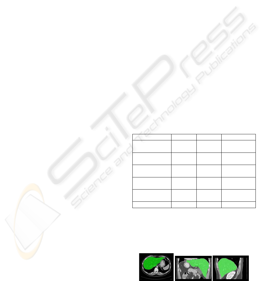
Figure 1: Best result obtained (left) axial view; (center)

coronal view; (right) sagittal view.

(a)

VISAPP 2009 - International Conference on Computer Vision Theory and Applications

158

The method attained a good performance in 17 of

the 20 exams, in which the overall score is above 65.

Figure 1 shows the result obtained in the best case,

with overall score of 82.05. It is possible to observe

that the liver boundaries are accurately defined.

In 3 exams, though, the results contain some

significant errors that can be verified visually. The

exam with the lowest score among all exams tested

has an overall score of 29.57. In this exam the liver

has a huge nodule, and it causes a leak of the

segmented region towards adjacent darker

structures. Considering the size of the nodule, the

result is reasonable, though.

On another exam with low score (46.18) it is

possible to observe a single major error, caused by a

peripheral nodule not classified as liver. This is

explained by the heuristic adopted, that considers a

single Gaussian curve to model liver tissue. Once the

nodule in this exam appears much darker than the

liver parenchyma, its voxel intensities lie outside the

range [TL,TH] defined by the Gaussian fit. As the

nodule is peripheral, it wasn’t possible to correct this

error with morphological fill holes, and therefore the

nodule region was not included in the final result.

Our results can be easily compared with many

other approaches, since the data and evaluation

metrics were obtained from the website of the liver

segmentation competition held in the Sliver07

conference, and the results of other approaches are

also available there. Thus, this comparison with

other works is straightforward once one visits the

conference’s website. If compared with other

automatic and semi-automatic methods, our method

has a good performance being ranked among the top

5 score.

6 CONCLUSIONS

We have presented a method to segment the liver

based on a level sets approach, using an evolutionary

method to estimate its optimal parameters. These

parameters were coded into genes of the individuals

of a GA, and the fitness evaluation was defined to

measure the similarity between a user defined

reference and the segmentation result.

Trough all the experiments it was possible to

verify the potential of the presented methodology.

The use of level sets, which is a consolidate

alternative to segment medical images, achieved

good performances in the tested exams, and the use

of GA to estimate its optimal parameters produced

robust parameters.

The method has, though, some limitations. It

presented some low performances in the presence of

peripheral nodules and veins, and also when nodules

with volume similar to the liver parenchyma were

observed. These cases were presented in details in

section 5.

It is important to notice that the method can be

applied to segment other organs beside the liver,

especially considering the ones roughly

homogeneous. In this case the GA would estimate

other parameters based on the input reference of the

organ to be segmented.

Some suggestions for further research would be a

better modelling to build the speed image

considering also the information of liver internal

structures, such as vessels and nodules. Another

possibility would be use the advection term to

suppress or reinforce some specific barriers, which

could be used to avoid leaking and also enable the

inclusion of peripheral nodules and veins in the final

result.

REFERENCES

Davis L. Handbook of Genetic Algorithms. Van Nostrand

Reinhold Company, New York, 1990.

Fujimoto H., Gu L., and Kaneko T., “Recognition of

abdominal organs using 3D mathematical

morphology,” Trans. Inst. Electron. Inf. Commun.

Eng. D-II, no. 5, pp. 843-850, May 2001.

Heimann T.; van Ginneken B.; Styner M.. "3D

Segmentation in the Clinic: A Grand Challenge",

(Eds.): 3D Segmentation in the Clinic: A Grand

Challenge, pp. 7-15, 2007.

Malladi, R. ,Sethian, J.A., Vemuri, B.C.. Shape modeling

with front propagation: a level set approach. IEEE

rans. Pattern Anal. Mach. Intell. 17 (2) 158–175, 1995.

Michalewicz Z (1994) Genetic Algorithms + Data

Structures = Evolution Pro-grams. Springer-Verlag,

Berlin Heidelberg New York

Lamecker H., Zachow S., Haberl H., Stiller M.. Medical

Applications for Statistical 3D Shape Models. Proc.

Computer Aided Surgery Around the Head, volume 17

of Fortschritt- Berichte VDI, p. 61, 2005.

Osher S., Sethian J. Fronts propagating with curvature-

dependent speed: algorithms based on Hamilton-

Jacobi formulations. J. Comput. Phys. 79 (1998) 12–

49.

Yoo T.S., Ackerman M. J., Lorensen W. E., Schroeder W.,

Chalana V., Aylward S., Metaxes D., Whitaker R..

Engineering and Algorithm Design for an Image

Processing API: A Technical Report on ITK - The

Insight Toolkit. In Proc. of Medicine Meets Virtual

Reality, J. Westwood, ed., IOS Press Amsterdam pp

586-592 (2002).

LIVER SEGMENTATION USING LEVEL SETS AND GENETIC ALGORITHMS

159