FAST APPROXIMATE NEAREST NEIGHBORS

WITH AUTOMATIC ALGORITHM CONFIGURATION

Marius Muja and David G. Lowe

Computer Science Department, University of British Columbia, Vancouver, B.C., Canada

Keywords:

Nearest-neighbors search, Randomized kd-trees, Hierarchical k-means tree, Clustering.

Abstract:

For many computer vision problems, the most time consuming component consists of nearest neighbor match-

ing in high-dimensional spaces. There are no known exact algorithms for solving these high-dimensional

problems that are faster than linear search. Approximate algorithms are known to provide large speedups with

only minor loss in accuracy, but many such algorithms have been published with only minimal guidance on

selecting an algorithm and its parameters for any given problem. In this paper, we describe a system that

answers the question, “What is the fastest approximate nearest-neighbor algorithm for my data?” Our system

will take any given dataset and desired degree of precision and use these to automatically determine the best

algorithm and parameter values. We also describe a new algorithm that applies priority search on hierarchical

k-means trees, which we have found to provide the best known performance on many datasets. After testing a

range of alternatives, we have found that multiple randomized k-d trees provide the best performance for other

datasets. We are releasing public domain code that implements these approaches. This library provides about

one order of magnitude improvement in query time over the best previously available software and provides

fully automated parameter selection.

1 INTRODUCTION

The most computationally expensive part of many

computer vision algorithms consists of searching for

the closest matches to high-dimensional vectors. Ex-

amples of such problems include ﬁnding the best

matches for local image features in large datasets

(Lowe, 2004; Philbin et al., 2007), clustering local

features into visual words using the k-means or sim-

ilar algorithms (Sivic and Zisserman, 2003), or per-

forming normalized cross-correlation to compare im-

age patches in large datasets (Torralba et al., 2008).

The nearest neighbor search problem is also of major

importance in many other applications, including ma-

chine learning, document retrieval, data compression,

bioinformatics, and data analysis.

We can deﬁne the nearest neighbor search prob-

lem as follows: given a set of points P = {p

,.. ., p

}

in a vector space X, these points must be preprocessed

in such a way that given a new query point q ∈ X,

ﬁnding the points in P that are nearest to q can be per-

formed efﬁciently. In this paper, we will assume that

X is an Euclidean vector space, which is appropriate

for most problems in computer vision. We will de-

scribe potential extensions of our approach to general

metric spaces, although this would come at some cost

in efﬁciency.

For high-dimensional spaces, there are often no

known algorithms for nearest neighbor search that

are more efﬁcient than simple linear search. As lin-

ear search is too costly for many applications, this

has generated an interest in algorithms that perform

approximate nearest neighbor search, in which non-

optimal neighbors are sometimes returned. Such ap-

proximate algorithms can be orders of magnitude

faster than exact search, while still providing near-

optimal accuracy.

There have been hundreds of papers published on

algorithms for approximate nearest neighbor search,

but there has been little systematic comparison to

guide the choice among algorithms and set their inter-

nal parameters. One reason for this is that the relative

performance of the algorithms varies widely based on

properties of the datasets, such as dimensionality, cor-

relations, clustering characteristics, and size. In this

paper, we attempt to bring some order to these re-

sults by comparing the most promising methods on

a range of realistic datasets with a wide range of di-

mensionality. In addition, we have developed an ap-

proach for automatic algorithm selection and conﬁgu-

331

Muja M. and G. Lowe D. (2009).

FAST APPROXIMATE NEAREST NEIGHBORS WITH AUTOMATIC ALGORITHM CONFIGURATION.

In Proceedings of the Fourth International Conference on Computer Vision Theory and Applications, pages 331-340

DOI: 10.5220/0001787803310340

 SciTePress

ration, which allows the best algorithm and parameter

settings to be determined automatically for any given

dataset. This approach allows for easy extension if

other algorithms are identiﬁed in the future that pro-

vide superior performance for particular datasets. Our

code is being made available in the public domain to

make it easy for others to perform comparisons and

contribute to improvements.

We also introduce an algorithm which modiﬁes

the previous method of using hierarchical k-means

trees. While previous methods for searching k-means

trees have used a branch-and-bound approach that

searches in depth-ﬁrst order, our method uses a pri-

ority queue to expand the search in order according to

the distance of each k-means domain from the query.

In addition, we are able to reduce the tree construc-

tion time by about an order of magnitude by limiting

the number of iterations for which the k-means clus-

tering is performed. For many datasets, we ﬁnd that

this algorithm has the highest known performance.

For other datasets, we have found that an algo-

rithm that uses multiple randomized kd-trees provides

the best results. This algorithm has only been pro-

posed recently (Silpa-Anan and Hartley, 2004; Silpa-

Anan and Hartley, 2008) and has not been widely

tested. Our results show that once optimal parame-

ter values have been determined this algorithm often

gives an order of magnitude improvement compared

to the best previous method that used a single kd-tree.

From the perspective of a person using our soft-

ware, no familiarity with the algorithms is neces-

sary and only some simple library routines are called.

The user provides a dataset, and our algorithm uses

a cross-validation approach to identify the best algo-

rithm and to search for the optimal parameter val-

ues to minimize the predicted search cost of future

queries. The user may also specify a desire to ac-

cept a less than optimal query time in exchange for

reduced memory usage, a reduction in data structure

build-time, or reduced time spent on parameter selec-

tion.

We demonstrate our approach by matching image

patches to a database of 100,000 other patches taken

under different illumination and imaging conditions.

In our experiments, we show it is possible to obtain

a speed-up by a factor of 1,000 times relative to lin-

ear search while still identifying 95% of the correct

nearest neighbors.

2 PREVIOUS RESEARCH

The most widely used algorithm for nearest-neighbor

search is the kd-tree (Freidman et al., 1977), which

works well for exact nearest neighbor search in low-

dimensional data, but quickly loses its effectiveness

as dimensionality increases. Arya et al. (Arya et al.,

1998) modify the original kd-tree algorithm to use

it for approximate matching. They impose a bound

on the accuracy of a solution using the notion of ε-

approximate nearest neighbor: a point p ∈ X is an ε-

approximate nearest neighbor of a query point q ∈ X,

if dist(p,q) ≤ (1 + ε)dist(p

∗

,q) where p

∗

is the true

nearest neighbor. The authors also propose the use of

a priority queue to speed up the search in a tree by

visiting tree nodes in order of their distance from the

query point. Beis and Lowe (Beis and Lowe, 1997)

describe a similar kd-tree based algorithm, but use a

stopping criterion based on examining a ﬁxed number

max

of leaf nodes, which can give better performance

than the ε-approximate cutoff.

Silpa-Anan and Hartley (Silpa-Anan and Hartley,

2008) propose the use of multiple randomized kd-

trees as a means to speed up approximate nearest-

neighbor search. They perform only limited tests, but

we have found this to work well over a wide range of

problems.

Fukunaga and Narendra (Fukunaga and Narendra,

1975) propose that nearest-neighbor matching be per-

formed with a tree structure constructed by clustering

the data points with the k-means algorithm into k dis-

joint groups and then recursively doing the same for

each of the groups. The tree they propose requires a

vector space because they compute the mean of each

cluster. Brin (Brin, 1995) proposes a similar tree,

called GNAT, Geometric Near-neighbor Access Tree,

in which he uses some of the data points as the cluster

centers instead of computing the cluster mean points.

This change allows the tree to be deﬁned in a general

metric space.

Liu et al. (Liu et al., 2004) propose a new kind

of metric tree that allows an overlap between the chil-

dren of each node, called the spill-tree. However, our

experiments so far have found that randomized kd-

trees provide higher performance while requiring less

memory.

Nister and Stewenius (Nister and Stewenius,

2006) present a fast method for nearest-neighbor fea-

ture search in very large databases. Their method is

based on accessing a single leaf node of a hierarchi-

cal k-means tree similar to that proposed by Fukunaga

and Narendra (Fukunaga and Narendra, 1975).

In (Leibe et al., 2006) the authors propose an efﬁ-

cient method for clustering and matching features in

large datasets. They compare several clustering meth-

ods: k-means clustering, agglomerative clustering,

and a combined partitional-agglomerative algorithm.

Similarly, (Mikolajczyk and Matas, 2007) evaluates

VISAPP 2009 - International Conference on Computer Vision Theory and Applications

332

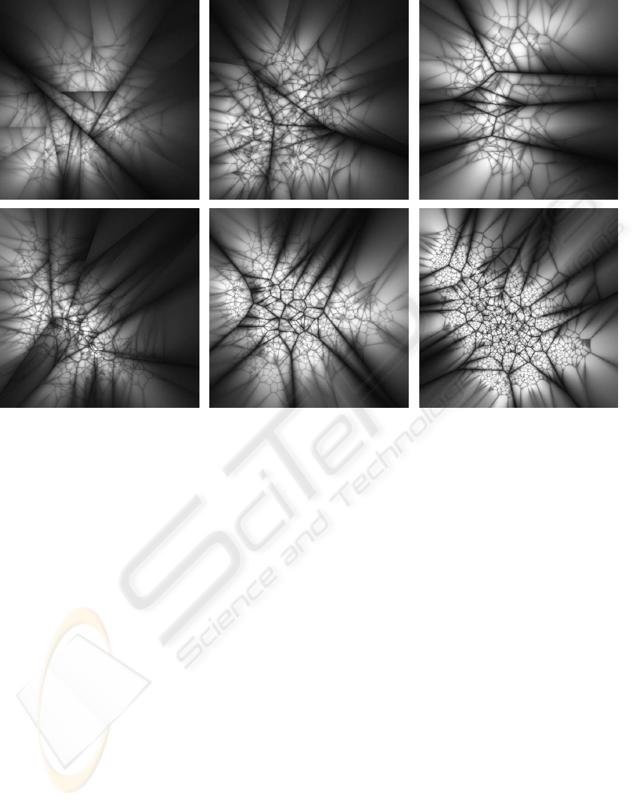
Figure 1: Projections of hierarchical k-means trees constructed using the same 100K SIFT features dataset with different

branching factors: 2, 4, 8, 16, 32, 128. The projections are constructed using the same technique as in (Schindler et al., 2007).

The gray values indicate the ratio between the distances to the nearest and the second-nearest cluster center at each tree level,

so that the darkest values (ratio≈1) fall near the boundaries between k-means regions.

the nearest neighbor matching performance for sev-

eral tree structures, including the kd-tree, the hierar-

chical k-means tree, and the agglomerative tree. We

have used these experiments to guide our choice of

algorithms.

3 FINDING FAST APPROXIMATE

NEAREST NEIGHBORS

We have compared many different algorithms for ap-

proximate nearest neighbor search on datasets with a

wide range of dimensionality. The accuracy of the ap-

proximation is measured in terms of precision, which

is deﬁned as the percentage of query points for which

the correct nearest neighbor is found. In our exper-

iments, one of two algorithms obtained the best per-

formance, depending on the dataset and desired pre-

cision. These algorithms used either the hierarchical

k-means tree or multiple randomized kd-trees. In this

section, we will begin by describing these algorithms.

We give comparisons to some other approaches in the

experiments section.

3.1 The Randomized kd-tree Algorithm

The classical kd-tree algorithm (Freidman et al.,

1977) is efﬁcient in low dimensions, but in high di-

mensions the performance rapidly degrades. To ob-

tain a speedup over linear search it becomes necessary

to settle for an approximate nearest-neighbor. This

improves the search speed at the cost of the algorithm

not always returning the exact nearest neighbors.

Silpa-Anan and Hartley (Silpa-Anan and Hartley,

2008) have recently proposed an improved version of

the kd-tree algorithm in which multiple randomized

kd-trees are created. The original kd-tree algorithm

splits the data in half at each level of the tree on the di-

mension for which the data exhibits the greatest vari-

ance. By comparison, the randomized trees are built

by choosing the split dimension randomly from the

ﬁrst D dimensions on which data has the greatest vari-

ance. We use the ﬁxed value D = 5 in our implemen-

tation, as this performs well across all our datasets and

does not beneﬁt signiﬁcantly from further tuning.

When searching the trees, a single priority queue

is maintained across all the randomized trees so that

FAST APPROXIMATE NEAREST NEIGHBORS WITH AUTOMATIC ALGORITHM CONFIGURATION

333

search can be ordered by increasing distance to each

bin boundary. The degree of approximation is deter-

mined by examining a ﬁxed number of leaf nodes, at

which point the search is terminated and the best can-

didates returned. In our implementation the user spec-

iﬁes only the desired search precision, which is used

during training to select the number of leaf nodes that

will be examined in order to achieve this precision.

3.2 The Hierarchical k-means Tree

Algorithm

The hierarchical k-means tree is constructed by split-

ting the data points at each level into K distinct re-

gions using a k-means clustering, and then apply-

ing the same method recursively to the points in

each region. We stop the recursion when the num-

ber of points in a region is smaller than K. Figure

1 shows projections of several hierarchical k-means

trees constructed from 100K SIFT features using dif-

ferent branching factors.

We have developed an algorithm that explores the

hierarchical k-means tree in a best-bin-ﬁrst manner,

by analogy to what has been found to improve the

exploration of the kd-tree. The algorithm initially

performs a single traversal through the tree and adds

to a priority queue all unexplored branches in each

node along the path. Next, it extracts from the prior-

ity queue the branch that has the closest center to the

query point and it restarts the tree traversal from that

branch. In each traversal the algorithm keeps adding

to the priority queue the unexplored branches along

the path. The degree of approximation is speciﬁed in

the same way as for the randomized kd-trees, by stop-

ping the search early after a predetermined number of

leaf nodes (dataset points) have been examined. This

parameter is set during training to achieve the user-

speciﬁed search precision.

We have experimented with a number of varia-

tions, such as using the distance to the closest Voronoi

border instead of the distance to the closest cluster

center, using multiple randomized k-means trees, or

using agglomerative clustering as proposed by Leibe

et al. (Leibe et al., 2006). However, these were found

not to give improved performance.

3.3 Automatic Selection of the Optimal

Algorithm

Our experiments have revealed that the optimal algo-

rithm for fast approximate nearest neighbor search is

highly dependent on several factors such as the struc-

ture of the dataset (whether there is any correlation

between the features in the dataset) and the desired

search precision. Additionally, each algorithm has a

set of parameters that have signiﬁcant inﬂuence on

the search performance. These parameters include the

number of randomized trees to use in the case of kd-

trees or the branching factor and the number of itera-

tions in the case of the hierarchical k-means tree.

By considering the algorithm itself as a parame-

ter of a generic nearest neighbor search routine, the

problem is reduced to determining the parameters that

give the best solution. This is an optimization prob-

lem in the parameter space. The cost is computed as

a combination of the search time, tree build time, and

tree memory overhead. Depending on the application,

each of these three factors has a different importance:

in some cases we don’t care much about the tree build

time (if we will build the tree only once and use it for

a large number of queries), while in other cases both

the tree build time and search time must be small (if

the tree is built on-line and searched a small number

of times). There are also situations when we wish to

limit the memory overhead. We control the relative

importance of each of these factors by using a build-

time weight, w

, and a memory weight, w

, to com-

pute the overall cost:

cost =

s+ w

(s+ w

opt

+ w

m (1)

where s represents the search time for the number of

vectors in the sample dataset, b represents the tree

build time, and m = m

represents the ratio of

memory used for the tree (m

) to the memory used

to store the data (m

The build-time weight (w

) controls the impor-

tance of the tree build time relative to the search time.

Setting w

= 0 means that we want the fastest search

time and don’t care about the tree build time, while

= 1 means that the tree build time and the search

time have the same importance. Similarly, the mem-

ory weight (w

) controls the importance of the mem-

ory overhead compared to the time overhead. The

time overhead is computed relative to the optimum

time cost (s+ w

opt

, which is deﬁned as the optimal

search and build time if memory usage is not a fac-

tor. Therefore, setting w

= 0 will choose the algo-

rithm and parameters that result in the fastest search

and build time without any regard to memory over-

head, while setting w

= 1 will give equal weight to

a given percentage increase in memory use as to the

same percentage increase in search and build time.

We choose the best nearest neighbor algorithm

and the optimum parameters in a two step approach:

a global exploration of the parameter space followed

by a local tuning of the best parameters. Initially,

we sample the parameter space at multiple points and

choose those values that minimize the cost of equation

VISAPP 2009 - International Conference on Computer Vision Theory and Applications

334

1. For this step we consider using {1,4,8, 16,32} as

the number of random kd-trees, {16,32,64,128,256}

as the branching factor for the k-means tree and

{1,5,10,15} as the number of k-means iterations. In

the second step we use the Nelder-Mead downhill

simplex method to further locally explore the param-

eter space and ﬁne-tune the best parameters obtained

in the ﬁrst step. Although this does not guarantee a

global minimum, our experiments have shown that

the parameter values obtained are close to optimum.

The optimization can be run on the full dataset or

just on a fraction of the dataset. Using the full dataset

gives the most accurate results but in the case of large

datasets it may take more time than desired. An op-

tion is provided to use just a fraction of the dataset

to select parameter values. We have found that using

just one tenth of the dataset typically selects parame-

ter values that still perform close to the optimum on

the full dataset. The parameter selection needs only

be performed once for each type of dataset, and our

library allows these values to be saved and applied to

all future datasets of the same type.

4 EXPERIMENTS

4.1 Randomized kd-trees

Figure 2 shows the value of searching in many ran-

domized kd-trees at the same time. It can be seen that

performance improves with the number of random-

ized trees up to a certain point (about 20 random trees

in this case) and that increasing the number of random

trees further leads to static or decreasing performance.

The memory overhead of using multiple random trees

increases linearly with the number of trees, so the cost

function may choose a lower number if memory us-

age is assigned importance.

4.2 Hierarchical k-means Tree

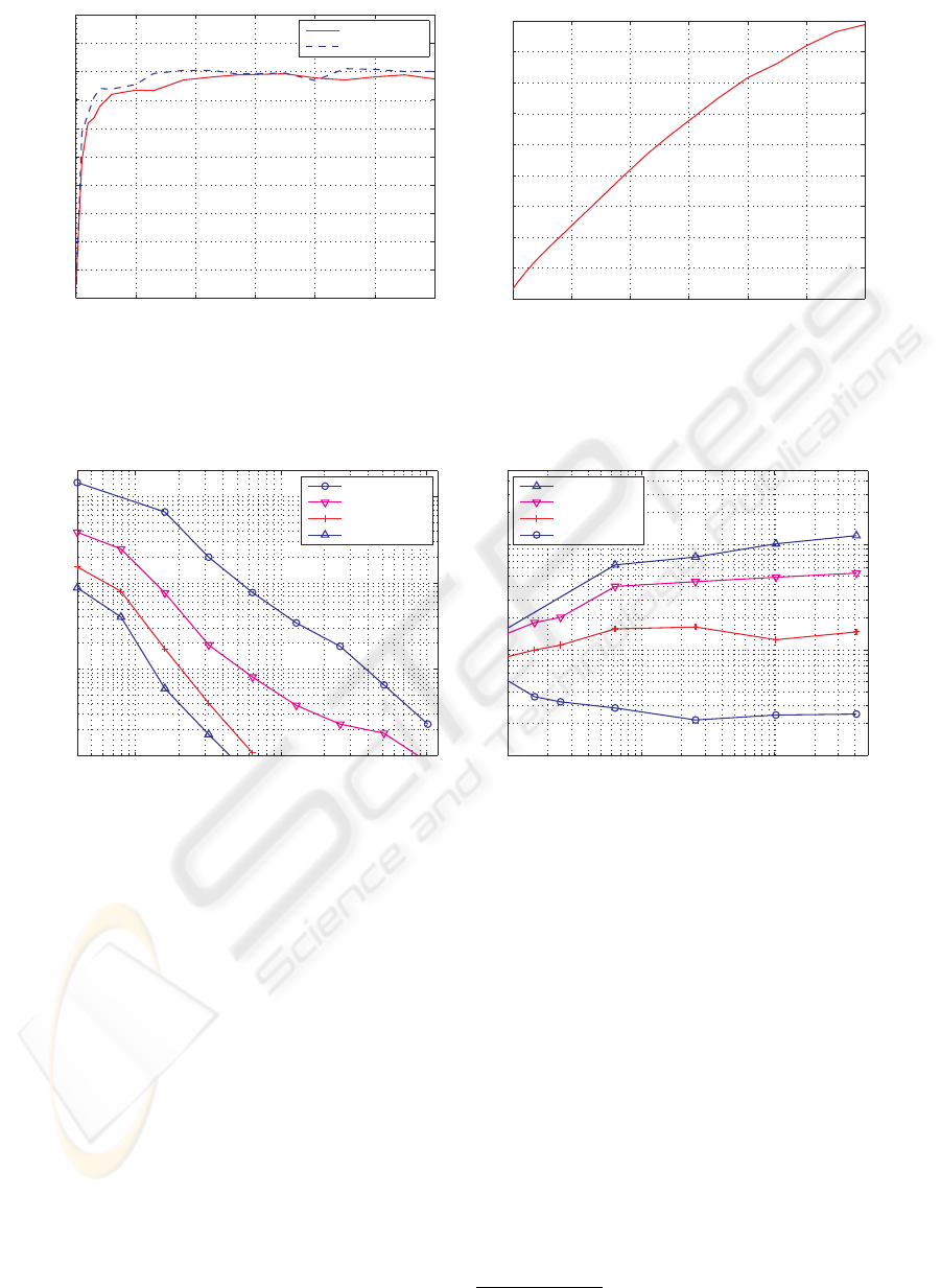
The hierarchical k-means tree algorithm has the high-

est performance for some datasets. However, one

disadvantage of this algorithm is that it often has a

higher tree-build time than the randomized kd-trees.

The build time can be reduced signiﬁcantly by doing

a small number of iterations in the k-means clustering

stage instead of running it until convergence. Figure 3

shows the performance of the tree constructed using a

limited number of iterations in the k-means clustering

step relative to the performance of the tree when the

k-means clustering is run until convergence. It can be

seen that using as few as 7 iterations we get more than

90% of the nearest-neighbor performance of the tree

Number of trees

Speedup over linear search

70% precision

95% precision

Figure 2: Speedup obtained by using multiple random kd-

trees (100K SIFT features dataset).

constructed using full convergence, but requiring less

than 10% of the build time.

When using zero iterations in the k-means cluster-

ing we obtain the more general GNAT tree of (Brin,

1995), which assumes that the data lives in a generic

metric space, not in a vector space. However ﬁgure

3(a) shows that the search performance of this tree is

worse than that of the hierarchical k-means tree (by

factor of 5).

4.3 Data Dimensionality

Data dimensionality is one of the factors that has a

great impact on the nearest neighbor matching per-

formance. Figure 4(a) shows how the search per-

formance degrades as the dimensionality increases.

The datasets each contain 10

vectors whose val-

ues are randomly sampled from the same uniform

distribution. These random datasets are one of the

most difﬁcult problems for nearest neighbor search,

as no value givesany predictive information about any

other value. As can be seen in ﬁgure 4(a), the nearest-

neighbor searches have a low efﬁciency for higher di-

mensional data (for 68% precision the approximate

search speed is no better than linear search when the

number of dimensions is greater than 800). However

real world datasets are normally much easier due to

correlations between dimensions.

The performance is markedly different for many

real-world datasets. Figure 4(b) shows the speedup

as a function of dimensionality for the Winder/Brown

image patches

resampled to achieve varying dimen-

sionality. In this case however, the speedup does not

decrease with dimensionality, it’s actually increasing

for some precisions. This can be explained by the

http://phototour.cs.washington.edu/patches/default.htm

FAST APPROXIMATE NEAREST NEIGHBORS WITH AUTOMATIC ALGORITHM CONFIGURATION

335

0 10 20 30 40 50 60

0.2

0.3

0.4

0.5

0.6

0.7

0.8

0.9

1.1

1.2

Iterations

Relative search performace

70% precision

95% precision

(a)

0 10 20 30 40 50 60

0.05

0.1

0.15

0.2

0.25

0.3

0.35

0.4

0.45

Relative tree construction time

Iterations

(b)

Figure 3: The inﬂuence that the number of k-means iterations has on the search time efﬁciency of the k-means tree (a) and on

the tree construction time (b) (100K SIFT features dataset).

Dimensions

Speedup over linear search

20% precision

68% precision

92% precision

98% precision

(a) Random vectors

Dimensions

Speedup over linear search

81% precision

85% precision

91% precision

97% precision

(b) Image patches

Figure 4: Search efﬁciency for data of varying dimensionality. The random vectors (a) represent the hardest case in which

dimensions have no correlations, while most real-world problems behave more like the image patches (b).

fact that there exists a strong correlation between the

dimensions, so that even for 64x64 patches (4096 di-

mensions), the similarity between only a few dimen-

sions provides strong evidence for overall patch simi-

larity.

Figure 5 shows four examples of queries on the

Trevi dataset of patches for different patch sizes.

4.4 Search Precision

The desired search precision determines the degree of

speedup that can be obtained with any approximate

algorithm. Looking at ﬁgure 6(b) (the sift1M dataset)

we see that if we are willing to accept a precision as

low as 60%, meaning that 40% of the neighbors re-

turned are not the exact nearest neighbors, but just

approximations, we can achievea speedup of three or-

ders of magnitude over linear search (using the mul-

tiple randomized kd-trees). However, if we require

a precision greater then 90% the speedup is smaller,

less than 2 orders of magnitude (using the hierarchical

k-means tree).

We use several datasets of different dimensions

for the experiments in ﬁgure 6. We construct a 100K

and 1 million SIFT features dataset by randomly sam-

pling a dataset of over 5 million SIFT features ex-

tracted from a collection of CD cover images (Nister

and Stewenius, 2006)

. These two datasets obtained

by random sampling have a relatively high degree of

difﬁculty in terms of nearest neighbour matching, be-

cause the features they contain usually do not have

http://www.vis.uky.edu/

stewe/ukbench/data/

VISAPP 2009 - International Conference on Computer Vision Theory and Applications

336

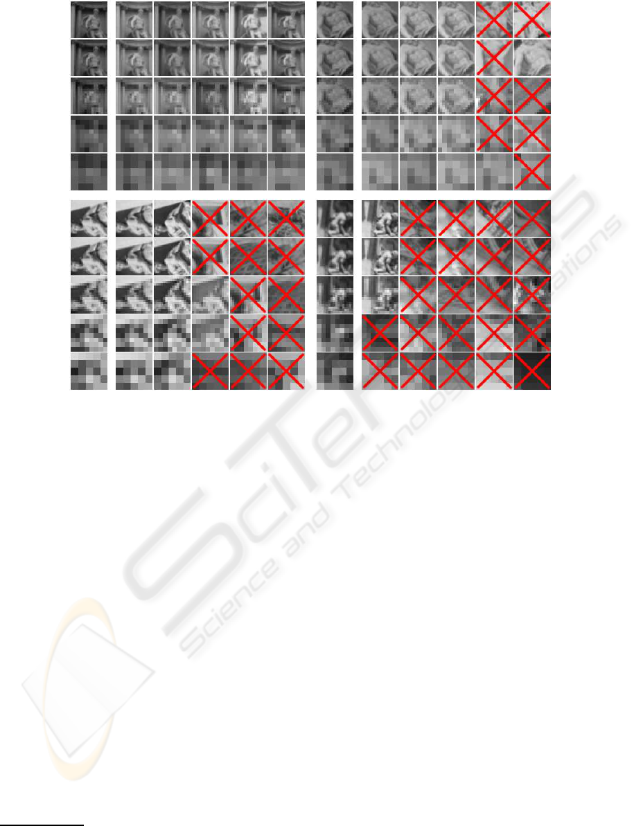
Figure 5: Examples of querying the Trevi Fountain patch dataset using different patch sizes. The query patch is on the left

of each panel, while the following 5 patches are the nearest neighbors from a set of 100,000 patches. Incorrect matches are

shown with an X.

“true” matches between them. We also use the en-

tire 31 million feature dataset from the same source

for the experiment in ﬁgure 6(b). Additionally we use

the patches datasets described in subsection 4.3 and

another 100K SIFT features dataset obtained from a

set of images forming a panorama.

We compare the two algorithmswe found to be the

best at ﬁnding fast approximate nearest neighbors (the

multiple randomized kd-trees and the hierarchical k-

means tree) with existing approaches, the ANN (Arya

et al., 1998) and LSH algorithms (Andoni, 2006)

the ﬁrst dataset of 100,000 SIFT features. Since the

LSH implementation (the E

LSH package) solves the

R-near neighbor problem (ﬁnds the neighbors within

a radius R of the query point, not the nearest neigh-

bors), to ﬁnd the nearest neighbors we have used the

approach suggested in the E

LSH’s user manual: we

compute the R-near neighbors for increasing values

of R. The parameters for the LSH algorithm were

chosen using the parameter estimation tool included

in the E

LSH package. For each case we have com-

puted the precision achieved as the percentage of the

We have used the publicly available implementations

of ANN (http://www.cs.umd.edu/

mount/ANN/) and LSH

(http://www.mit.edu/

andoni/LSH/)

query points for which the nearest neighbors were

correctly found. Figure 6(a) shows that the hierar-

chical k-means algorithm outperforms both the ANN

and LSH algorithms by about an order of magnitude.

The results for ANN are consistent with the experi-

ment in ﬁgure 2, as ANN uses only a single kd-tree

and does not beneﬁt from the speedup due to using

multiple randomized trees.

Figure 6(b) shows the performance of the random-

ized kd-trees and the hierarchical k-means on datasets

of different sizes. The ﬁgure shows that the two algo-

rithms scale well with the increase in the dataset size,

having the speedup over linear search increase with

the dataset size.

Figure 6(c) compares the performance of near-

est neighbor matching when the dataset contains true

matches for each feature in the test set to the case

when it contains false matches. In this experiment we

used the two 100K SIFT features datasets described

above. The ﬁrst is randomly sampled from a 5 million

SIFT features dataset and it contains false matches

for each feature in the test set. The second contains

SIFT features extracted from a set of images forming

a panorama. These features were extracted from the

overlapping regions of the images, and we use only

FAST APPROXIMATE NEAREST NEIGHBORS WITH AUTOMATIC ALGORITHM CONFIGURATION

337

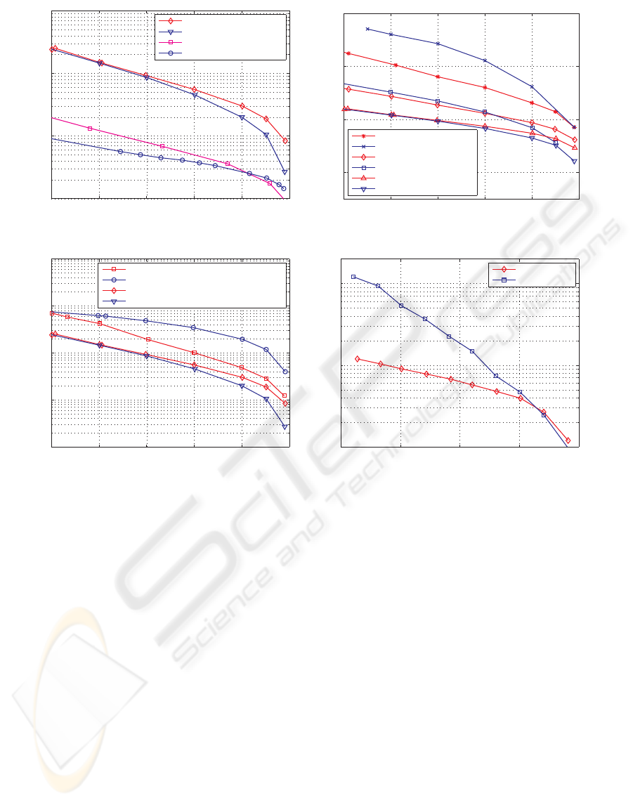
50 60 70 80 90 100

Correct neighbors (%)

Speedup over linear search

k−means tree − sift 100K

rand. kd−trees − sift 100K

ANN − sift 100K

LSH − sift 100K

(a)

50 60 70 80 90 100

Correct neighbors (%)

Speedup over linear search

k−means tree − sift 31M

rand. kd−trees − sift 31M

k−means tree − sift 1M

rand. kd−trees − sift 1M

k−means tree − sift 100K

rand. kd−trees − sift 100K

(b)

50 60 70 80 90 100

Correct neighbors (%)

Speedup over linear search

k−means tree − sift 100K true matches

rand. kd−trees − sift 100K true matches

k−means tree − sift 100K false matches

rand. kd−trees − sift 100K false matches

(c)

80 85 90 95 100

Correct neighbors (%)

Speedup over linear search

k−means tree

rand. kd−trees

(d)

Figure 6: Search efﬁciency. (a) Comparison of different algorithms. (b) Search speedup for different dataset sizes. (c) Search

speedup when the query points don’t have “true” matches in the dataset vs the case when they have. (d) Search speedup for

the Trevi Fountain patches dataset.

those that have a true match in the dataset. Our ex-

periments showed that the randomized kd-trees have

a signiﬁcantly better performance for true matches,

when the query features are likely to be signiﬁcantly

closer than other neighbors. Similar results were re-

ported in (Mikolajczyk and Matas, 2007).

Figure 6(d) shows the difference in performance

between the randomized kd-trees and the hierarchical

k-means tree for one of the Winder/Brown patches

dataset. In this case, the randomized kd-trees algo-

rithm clearly outperforms the hierarchical k-means al-

gorithm everywhere except for precisions very close

to 100%. It appears that the kd-tree works much better

in cases when the intrinsic dimensionality of the data

is much lower than the actual dimensionality, pre-

sumably because it can better exploit the correlations

among dimensions. However, Figure 6(b) shows that

the k-means tree can perform better for other datasets

(especially for high precisions). This shows the im-

portance of performing algorithm selection on each

dataset.

4.5 Automatic Algorithm and

Parameter Selection

In table 1, we show the results from running the pa-

rameter selection procedure described in 3.3 on the

dataset containing 100K random sampled SIFT fea-

tures. We have used two different search precisions

(60% and 90%) and several combinationsof the trade-

off factors w

and w

. For the build time weight,

, we used three different possible values: 0 rep-

resenting the case where we don’t care about the tree

build time, 1 for the case where the tree build time

and search time have the same importance and 0.01

representing the case where we care mainly about the

search time but we also want to avoid a large build

time. Similarly, the memory weight was chosen to be

VISAPP 2009 - International Conference on Computer Vision Theory and Applications

338

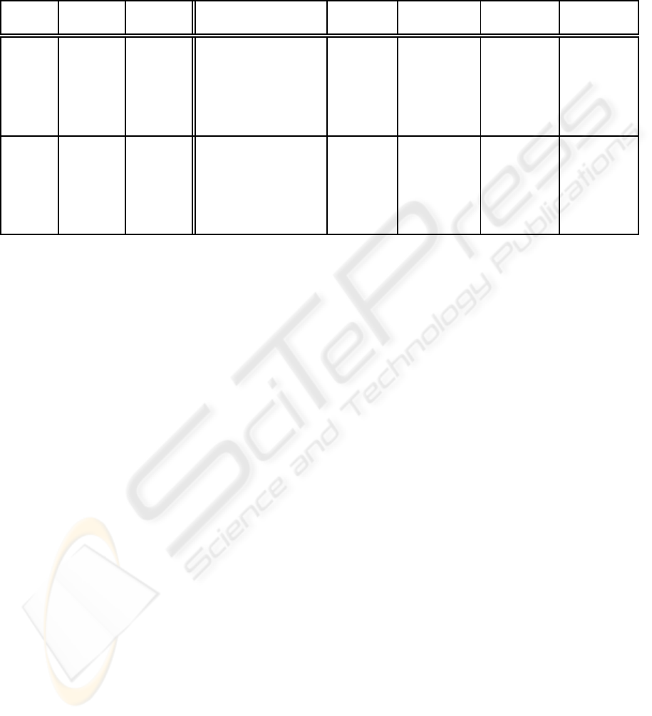
Table 1: The algorithms chosen by our automatic algorithm and parameter selection procedure (sift100K dataset). The

“Algorithm” column shows the algorithm chosen and its optimum parameters (number of random trees in case of the kd-tree;

branching factor and number of iterations for the k-means tree), the “Dist. Error” column shows the mean distance error

compared to the exact nearest neighbors, the “Search Speedup” shows the search speedup compared to linear search, the

“Memory Used” shows the memory used by the tree(s) as a fraction of the memory used by the dataset and the “Build Time”

column shows the tree build time as a fraction of the linear search time for the test set.

Pr.(%) w

Algorithm Dist.

Error

Speedup

Memory

Used

Build

Time

60%

0 0 k-means, 16, 15 0.096 181.10 0.51 0.58

0 1 k-means, 32, 10 0.058 180.9 0.37 0.56

0.01 0 k-means, 16, 5 0.077 163.25 0.50 0.26

0.01 1 kd-tree, 4 0.041 109.50 0.26 0.12

1 0 kd-tree,1 0.044 56.87 0.07 0.03

* ∞ kd-tree,1 0.044 56.87 0.07 0.03

90%

0 0 k-means, 128, 10 0.008 31.67 0.18 1.82

0 1 k-means, 128, 15 0.007 30.53 0.18 2.32

0.01 0 k-means, 32, 5 0.011 29.47 0.36 0.35

1 0 k-means, 16, 1 0.016 21.59 0.48 0.10

1 1 kd-tree,1 0.005 5.05 0.07 0.03

* ∞ kd-tree,1 0.005 5.05 0.07 0.03

0 for the case where the memory usage is not a con-

cern, ∞ representing the case where the memory use

is the dominant concern and 1 as a middle ground be-

tween the two cases.

Examining table 1 we can see that for the cases

when the build time or the memory overhead had the

highest weight, the algorithm chosen was the kd-tree

with a single tree because it is both the most memory

efﬁcient and the fastest to build. When no importance

was given to the tree build time and the memory over-

head the algorithm chosen was k-means, as conﬁrmed

by the plots in ﬁgure 6(b). The branching factors and

the number of iterations chosen for the k-means al-

gorithm depend on the search precision and the tree

build time weight: higher branching factors proved to

have better performance for higher precisions and the

tree build time increases when the branching factor or

the number of iterations increase.

5 CONCLUSIONS

In the approach described in this paper, automatic al-

gorithm conﬁguration allows a user to achieve high

performance in approximate nearest neighbor match-

ing by calling a single library routine. The user need

only provide an example of the type of dataset that

will be used and the desired precision, and may op-

tionally specify the importance of minimizing mem-

ory or build time rather than just search time. All re-

maining steps of algorithm selection and parameter

optimization are performed automatically.

In our experiments, we have found that either of

two algorithms can have the best performance, de-

pending on the dataset and desired precision. One of

these is an algorithm we have developed that com-

bines two previous approaches: searching hierarchi-

cal k-means trees with a priority search order. The

second method is to use multiple randomized kd-

trees. We have demonstrated that these can speed the

matching of high-dimensional vectors by up to sev-

eral orders of magnitude compared to linear search.

The use of automated algorithm conﬁguration will

make it easy to incorporate any new algorithms that

are found in the future to have superior performance

for particular datasets. We intend to keep adding new

datasets to our website and provide test results for

further algorithms. Our public domain library will

enable others to perform detailed comparisons with

new approaches and contribute to the extension of this

software.

ACKNOWLEDGEMENTS

This research has been supported by the Natural Sci-

ences and Engineering Research Council of Canada

and by the Canadian Institute for Advanced Research.

We wish to thank Matthew Brown, Richard Hartley,

Scott Helmer, Hoyt Koepke, Sancho McCann, Panu

Turcot and Andrew Zisserman for valuable discus-

sions and usefull feedback regarding this work.

FAST APPROXIMATE NEAREST NEIGHBORS WITH AUTOMATIC ALGORITHM CONFIGURATION

339

REFERENCES

Andoni, A. (2006). Near-optimal hashing algorithms for ap-

proximate nearest neighbor in high dimensions. Pro-

ceedings of the 47th Annual IEEE Symposium on

Foundations of Computer Science (FOCS’06), pages

459–468.

Arya, S., Mount, D. M., Netanyahu, N. S., Silverman, R.,

and Wu, A. Y. (1998). An optimal algorithm for ap-

proximate nearest neighbor searching in ﬁxed dimen-

sions. Journal of the ACM, 45:891–923.

Beis, J. S. and Lowe, D. G. (1997). Shape indexing using

approximate nearest-neighbor search in high dimen-

sional spaces. In CVPR, pages 1000–1006.

Brin, S. (1995). Near neighbor search in large metric

spaces. In VLDB, pages 574–584.

Freidman, J. H., Bentley, J. L., and Finkel, R. A. (1977).

An algorithm for ﬁnding best matches in logarithmic

expected time. ACM Trans. Math. Softw., 3:209–226.

Fukunaga, K. and Narendra, P. M. (1975). A branch and

bound algorithm for computing k-nearest neighbors.

IEEE Trans. Comput., 24:750–753.

Leibe, B., Mikolajczyk, K., and Schiele, B. (2006). Efﬁ-

cient clustering and matching for object class recogni-

tion. In BMVC.

Liu, T., Moore, A., Gray, A., and Yang, K. (2004). An inves-

tigation of practical approximate nearest neighbor al-

gorithms. In Neural Information Processing Systems.

Lowe, D. G. (2004). Distinctive image features from scale-

invariant keypoints. Int. Journal of Computer Vision,

60:91–110.

Mikolajczyk, K. and Matas, J. (2007). Improving descrip-

tors for fast tree matching by optimal linear projection.

In Computer Vision, 2007. ICCV 2007. IEEE 11th In-

ternational Conference on, pages 1–8.

Nister, D. and Stewenius, H. (2006). Scalable recognition

with a vocabulary tree. In CVPR, pages 2161–2168.

Philbin, J., Chum, O., Isard, M., Sivic, J., and Zisserman, A.

(2007). Object retrieval with large vocabularies and

fast spatial matching. In CVPR.

Schindler, G., Brown, M., and Szeliski, R. (2007). City-

scale location recognition. In CVPR, pages 1–7.

Silpa-Anan, C. and Hartley, R. (2004). Localization us-

ing an imagemap. In Australasian Conference on

Robotics and Automation.

Silpa-Anan, C. and Hartley, R. (2008). Optimised KD-trees

for fast image descriptor matching. In CVPR.

Sivic, J. and Zisserman, A. (2003). Video Google: A text

retrieval approach to object matching in videos. In

ICCV.

Torralba, A., Fergus, R., and Freeman, W. T. (2008). 80

million tiny images: A large data set for nonpara-

metric object and scene recognition. IEEE Transac-

tions on Pattern Analysis and Machine Intelligence,

30(11):1958–1970.

VISAPP 2009 - International Conference on Computer Vision Theory and Applications

340