
TEMPORAL VIDEO COMP
R
ESSION USING MODE FACTOR
AND POLYNOMIAL FITTING ON WAVELET COEFFICIENTS
T. Nithyaletchumy Devi, W. K. Lim, W. N. Tan, Y. F. Tan, H. T. Teng
Faculty of Engineering, Multimedia University, 63100 Cyberjaya, Selangor, Malaysia
Y. F. Chang
Faculty of Information and Communication Technology, Universiti Tunku Abdul Rahman
46200 Petaling Jaya, Selangor, Malaysia
Keywords: Temporal video compression, Wavelet transform, Haar wavelet, Polynomial fitting.
Abstract: The core idea of this study is to build an algorithm that functions to compress video sequences. The mode
value at every pixel along the temporal direction is calculated. If the frequency of the mode value satisfies a
predetermined frequency, then the intensity values for entire entries at that particular pixel position will be
changed to the mode value. The wavelet techniques will be applied to the pixels that do not satisfy the
predetermined frequency and followed by a polynomial fitting method. For the purpose of compression,
only the polynomial coefficients for pixels that do not satisfy the predetermined frequency, the mode values
for pixels that satisfy the predetermined frequency and the corresponding pixel positions will be stored. To
decompress, wavelet coefficients are estimated by the respective polynomials. The intensity values at the
intended pixel position are obtained by inverse wavelet transform for pixels that do not satisfy the
predetermined frequency. On the other hand, the stored mode values will be used to represent the intensity
values throughout the time interval. This method portrays a prospect to achieve an acceptable
decompressed video quality and compression ratio.
1 INTRODUCTION
On the whole, video compression denotes an act to
represent the details of a video sequence by means
of minimal data. Instead of transmitting all the
images, a code of the image representation will be
transmitted with a much smaller data size (Symes,
P.D., 2001). Furthermore, data can be compressed
before storage and transmission and decompressed
at the receiver, besides increasing the bandwidth
available (Symes, P.D., 2003). The two main
classification of compression are the lossless
compression and the lossy compression. These
methods have two main strategies, namely,
redundancy and irrelevancy respectively. In lossless
compression, the concentration is on obtaining
efficient ways of encoding the data. Additionally,
there will be no information that is irretrievably lost
in the process and it is exactly reversible. Whereas,
lossy compression transforms the image to have
simplified information and removes the data that we
can’t perceive in order to attain reduction in the file
size. It is an irreversible process that permanently
disposes some information. There are formats that
allow compression to as little as 1% but too much
compression may be dreadful as the changes
becomes visible and observable which can also
result to a video that can be hardly recognized
(Dunn, R.D., 2002).
Wavelet has extensively inspired both image and
video compression (Averbuch, A., 1996,
Koornwinder, T.H., 1993). With this basis, our
approach is to apply wavelet, to be precise, Haar, in
the temporal direction. The quintessence of this
study is to seek an algorithm to compress by
extracting only the perceptible element, thus
considerably reducing the data needed to be stored
whilst maintaining the adequate image quality.
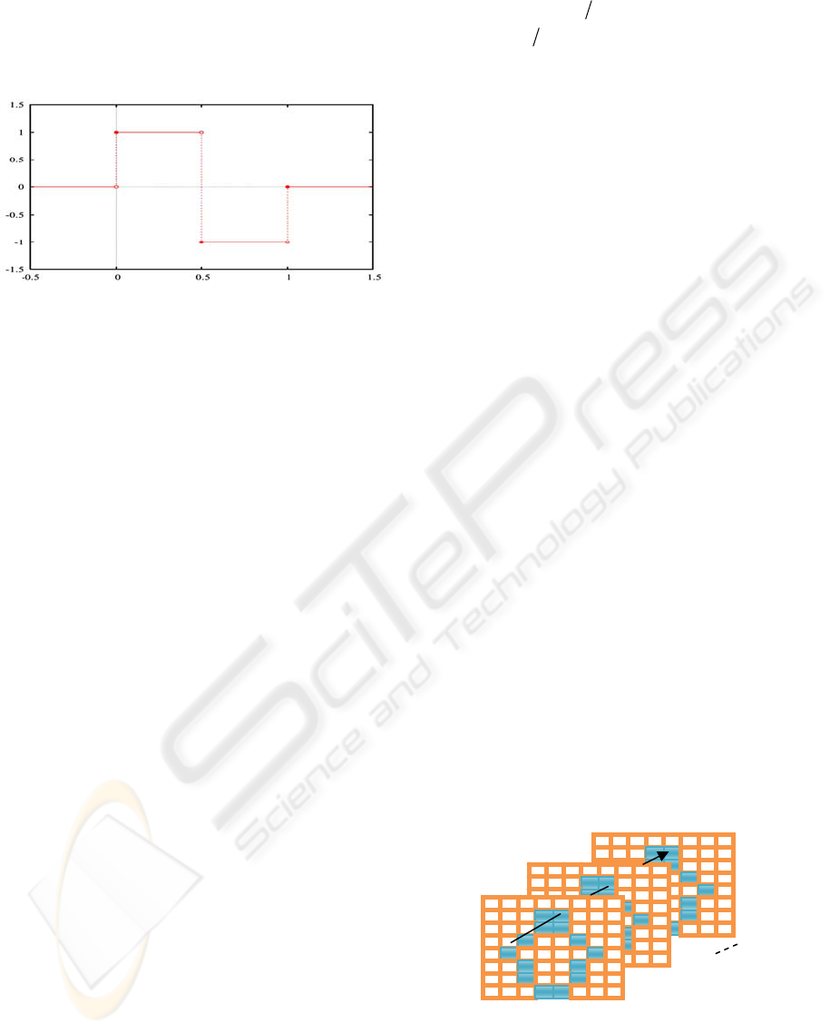
Previously, the wavelet decomposition coefficients
which were generated using the Haar wavelet
(Figure 1) were applied on the pixel intensity values
160
Nithyaletchumy Devi T., Lim W., Tan W., Tan Y., Teng H. and Chang Y. (2009).
TEMPORAL VIDEO COMPRESSION USING MODE FACTOR AND POLYNOMIAL FITTING ON WAVELET COEFFICIENTS.
In Proceedings of the Fourth International Conference on Computer Vision Theory and Applications, pages 160-165
DOI: 10.5220/0001787901600165
Copyright
c
SciTePress
at all pixel positions and were approximated by a
polynomial of a fixed degree (T. Nithyaletchumy
Devi et al., 2008). It is a hybrid method with an
interest of wavelet related to a polynomial fitting.
Figure 1: The Haar Wavelet
()
t
ψ
.
In this study, the mode value at each pixel
position along the temporal direction is calculated.
Subsequently, the frequency of the mode value will
be compared to a predetermined percentage. Having
the acceptable value of frequency, substitutes all the
intensity values at the pixel position along the
temporal direction to have the mode value and stores
a single mode value for the entire temporal
direction. Pixel positions that did not satisfy the
predetermined frequency will have wavelet applied
on to obtain the wavelet decomposition coefficient
using the Haar wavelet and followed by polynomial
fitting of a fixed degree. Only the coefficients of the
polynomials at apiece pixel along the temporal
direction, the mode values for the pixels that satisfy
the predetermined frequency and the corresponding
pixel positions will be stored for the purpose of
compression. The decompression is done by
estimating the wavelet coefficients from the
polynomials with the stored coefficients and
retrieving the mode values at intended pixel position
throughout the time interval.
Even though, there are a wide variety of popular
wavelet algorithms such as the Daubechies wavelets,
Mexican Hat wavelets and Morlet wavelets which
have the advantage of better resolution for smoothly
changing motions but they are more expensive to
calculate than the Haar wavelets (Kaplan, I., 2004).
The Haar wavelet transform is theoretically trouble-
free and speedy, exactly reversible and handles well
over the edge effects that are a problem with other
wavelet transforms.
The Haar wavelet’s mother wavelet function
()
t
ψ
and its scaling function
()
t
φ
are as described
below. Without loss of generality, we shall use the
same symbols for normalized wavelet and scaling
functions.
()
⎪
⎩
⎪
⎨
⎧
−=
0
1
1
t
ψ
otherwise
,121
,210
<≤
<
≤
t
t
and
()
⎩
⎨
⎧
=
0
1
t
φ
otherwise
,10
<
≤ t
2 TEMPORAL COMPRESSION
AND DECOMPRESSION
In order to understand ways to modify an image, it is
only essential to master the way the computer stores
the image. Consider a
T
H
M
××
pixel gray scale
image, where
H
M
×
, the size of each frame and
T
,
the total number of frames considered. The
computer stores this image as a
H
M
×
matrix, with
each elements ranging from 0 to 255. At this
primary level,
T
is best sustained at powers of two
(e.g. 2, 4, 8, 16 etc.) as to permit a straight forward
distribution of data without any additional
manipulation as far as wavelet is concern.
In this study, first and foremost task is to
calculate the mode, denoted as , at each pixel
location
ij
q
(
)
ji, along the temporal direction. Let
be the corresponding frequency of . For each
ij
fr
ij
q
(
)
ji, , if
(
)
Tp ×%fr
ij
≥
, 1000 ≤
<
p , then the pixel
location
(
)
ji,
2
will be stored in set , else it will be
in set
S . For each pixel location
(
in set ,
all intensity values along the temporal direction will
be changed to . For each pixel location
1
S
)
ji,
1
S
ij
q
(
)
ji,
2
S
in
set , Haar wavelet decomposition method will be
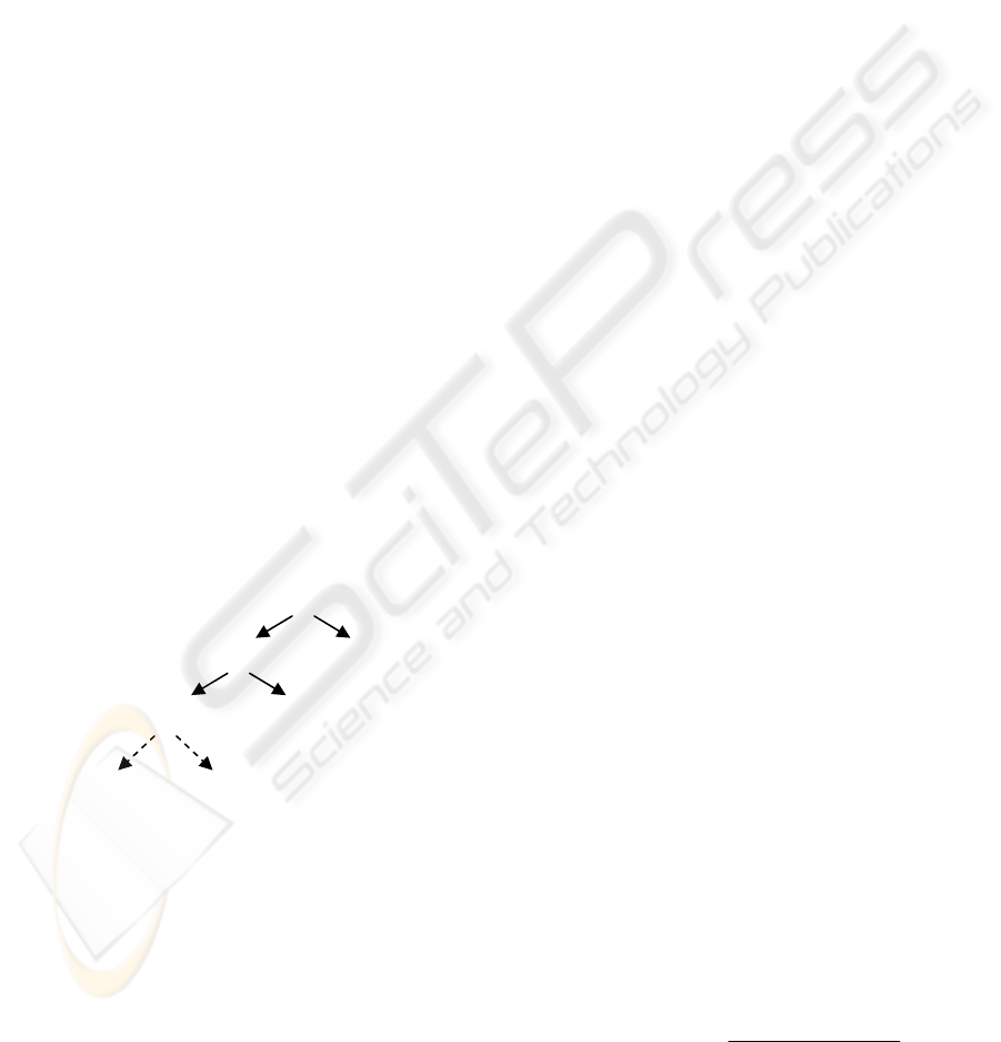
applied. Illustrating this in a pictorial form (see
Figure 2 below), the pixel positions in set are not
shaded, whereas the pixel positions in set are
denoted by the shaded boxes.
2
S
1
S
Figure 2: The pixel positions in set are not shaded,
whereas the pixel positions in set are shaded.
1
S
2
S
Consider the pixels in , identify the intensity
values at the pixel position at every frame as
2
S
i,
()
j
t=T
t
=
2
t
=
1
TEMPORAL VIDEO COMPRESSION USING MODE FACTOR AND POLYNOMIAL FITTING ON WAVELET
COEFFICIENTS
161
()
{
}
t
and for each
()
ji,
perform Haar wavelet
decomposition to the sequen
()
c
ij
,
ce
{
}
tc
ij
for n levels,
Nn ,...,2,1= :
()
,
1
∑∑∑
−
−nNk
ij
kna
where
()
()
()
2,2 ∈−−+−
=
−
N
qk
q
ij
nN
ktkqNdkt
ψφ
where
,
1
∑
−
−=
N
nN
qN
wv +
−n
,n
q
K
()
()
,
,
−
∑
∑
kqNd
kna
k
ij
k
ij
φ
are the orthogonal subsp
ction space.
()
()
2
⎭
⎬
⎫
⎭
⎬
⎫
k 1−− N
, = Nq
aces of the
2 −
−
−
t
kt
q
nN
ψ
⎩
⎨
⎧
=
⎩
w
q
of our fun
⎨
⎧
=
−
v
nN
decomposition
Two sets of coefficients, which are, the
approximation coefficients
()
{
}
ta
ij
,1
and the detail
coefficients
()
{
}
td
ij
,1 will be generated as shown in
Figure 3. Subsequently Haar wavelet
decomposition is reiterated to the approximation
coefficients sequence
()
, the
{
}
ta
ij
,1
and obtain the
sequences
()
{
}
ta
ij
,2 and
()
{
}
td
ij
,2 . This procedure
is persisted for say,
N nu times whereby N
signifies th f the decomposition and
it is depending on our preference. This will affect
the file size and quality which is the trade-off that
we will have to decide on.
m
wa
avelet d
ber
vel
e w
h
of
et
ecomposition
e
e level o
Figure 3: Th
means of both t
By
sequen
tree.
detail coefficients
ces
() ( )
{
}
tNdtd
ijij
,,,,1 K and the
approximation coefficients sequence
()
{
}
tNa
ij
, , the
original sequence
()
{
}
t
ly s
esse
c
ij
can be re
l
l
ass
u
emble We
notice that the detail coefficients incl erous
values that are liter mall, predominantly due to
pixels comprising r movements along the
temporal direction. Then, we calculate the
cumulative values for the approximation coefficients
and the absolute values of the detail coefficients to
retain an increasing trend respectively. With that,
we are able to fit the cumulative values of the
respective coefficients using linear combinations of
polynomials of degree
1
d.
de num
a
−
R
as follows:
1
1
−
=
∑
r
R
r
r
ij
tb
(1)
where are constant resolved for a prefe
value o
r
ij
b
f
r
s to be rred
R,,2,1 K
=
.
l
For storage purpose,
ij
q
is stored for each pixel
location i d the cn set an orresponding values of
1
S
p
r
ij
b
for fitted polynomia on approximation and
detail coefficients are stored for each pixel location
in set
2
S . For decompression purposes, the intensity
values along temporal direction for each pixel
location in set
1
S are assigned the values of
ij
q .
For each pixel location in set
2
S , the cumulative
values for both a proximation coefficients and detail
coefficients at any frame
t
,
[]
Tt ,1∈
can then be
estimated from the polynomial in
()
1 . Utilizing
these estimated cumulative values, we are able to
reconstruct the corresponding intensity values in a
lossy manner.
3 RESULTS A DISCUSSION
ell-
of
ND
We tested the current study’s method using a w
known video sequence, “Akiyo”, with frame size
144176
×
pixels. Th o was independently
different d
is vide
scrutinized through first 16 and first 32 frames for
various
p at different levels of wavelets and fitted on
egrees of polynomial. Outcome of each
circumstance demonstrates the significance of the
role played by numbers of frames, frequency of
mode, level of the wavelet and degrees of
polynomial. The ensuing data are then compressed
using the discussed method, saved for
decompression and consequently the peak signal to
noise ratio (
PSNR) (Taubman, D.S. et al., 2002) of
each frame are computed using the following
formula.
⎟
⎟
⎞
⎜
⎛
255
2
PSN
()
tc
ij
()
t,1
ij
a
ij
()
t,2
()
tNd
ij
,
ij
()
t,2
⎠
⎜
⎝
=
Error SquareMean
log10
10
R
()
t,1d
a
()
tNa
ij
,
d
ij
VISAPP 2009 - International Conference on Computer Vision Theory and Applications
162
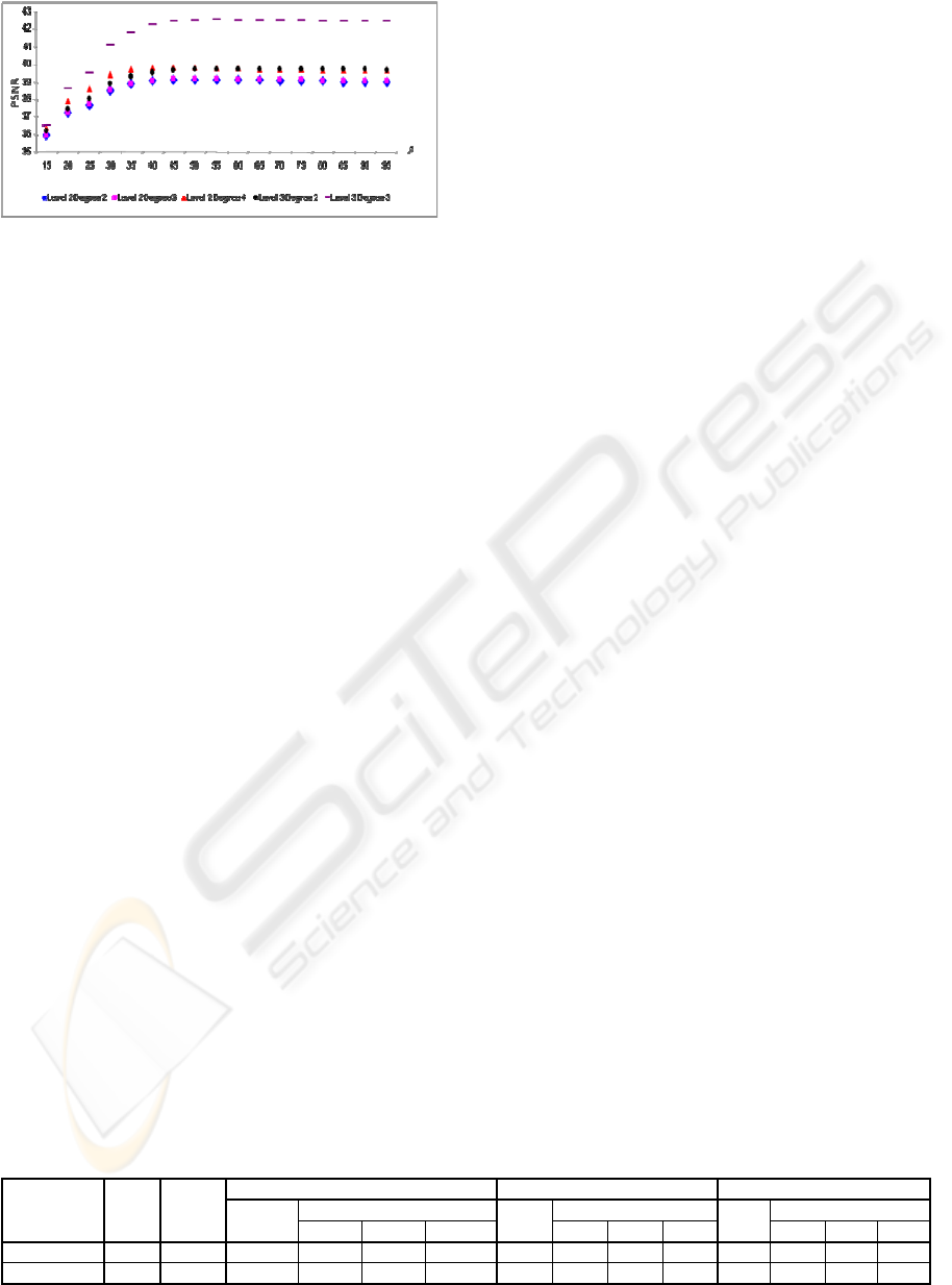
Figure 4: PSNR versus p using the first 32 frames at level
2 and 3 of wavelet decomposition and different degree of
polynomial fitting.
sition level 2 and 3 at degree 2, 3
and 4. Prominently, for both 16 and 32 frames,
diff 2
sition process and the
pixels that
um, maximum and mean values of
PS
mpo
Pre
: Result using the current study’s method
mode to be at least of the
to l
es used (16 and 32
polynomial degree (degree 2, 3 and
Size : Size of the information needed to be
e
PSNR : PSNR of each scenario
g the first 16 frames using p = 25, 50 and 75 at different levels
File Size (KB) Average PSNR CR
Figure 4 shows the PSNR versus p for p
ranging from 5 to 95, for 32 frames using Haar
wavelet decompo
erent degrees used for polynomial at level
wavelet decomposition does not bring significant
improvement in the
PSNR, whereas for 32 frames,
different degrees used for polynomial at level 3
shows a more significant improvement in the
PSNR.
Perhaps, this is due to the fact that a degree 3
polynomial fit exactly to the 4 data obtained on the
approximation coefficients.
The
p chosen is vital as it ascertains the
stringency on the minimum frequency that needed to
be obtained to segregate between pixels that go
through the wavelet decompo
will have all intensity values surrogated
with the mode value. From Figure 3, the optimum
p lies between 45 to 55 for the tested set of
parameters.
The degree chosen at each scenario is also
important because as the level of wavelet and degree
of polynomial increase, the number of data
concerned in generating the approximation
coefficients should possibly consist of at least the
minimum number of data needed to evaluate the
coefficients on that particular degree of polynomial.
This is an essential rule of thumb for analyzing
rationales. For an instance, applying a level 3
wavelet using the first 16 frames, it is not suitable to
use a degree 3 polynomial for its fitting as there will
only be two approximation coefficients, conversely,
we can do so using the first 32 frames.
Alternatively, in order to use a level of wavelet
decomposition that is higher than the number of data
obtained at the approximation coefficients, we may
chose to apply a lower degree of polynomial to the
approximation coefficients and a higher degree of
polynomial to the detail coefficients. This allows us
to evaluate the scenarios at a higher level but of
course with a natural increase in the file size bearing
in mind that higher polynomials produce more
coefficients.
The minim
Table 1: Minimum, maximum and mean values of PSNR usin
of wavelet and degrees of polynomial.
NR of each scenario are tabulated in Table 1
(using the first 16 frames) and Table 2 (using the
first 32 frames) in comparison with our previous
study’s method (T. Nithyaletchumy Devi et al.,
2008) and current study’s method, with
p = 25, 50
and
75 . In the previous method, the wavelet
deco sition coefficients were generated from the
pixel intensity values at all pixel positions. Then,
these coefficients were estimated by a polynomial of
a fixed degree at every pixel positions. The current
method on the other hand, applies polynomial fitting
only at pixel positions whereby the predetermined
frequency is not satisfied. By design, this reduces
the amount of information to be saved which has a
direct impinge on file size and compression ratio.
Information in the tables includes the following:
vious : Results using the previous study’s
method (wavelet applied to all pixel intensity
values)
Current
(conversed method)
p : Frequency of %p
ta number frames involved
Frames : Number of fram
frames)Level : The wavelet decomposition level
(level 2 and 3)
Degree : The
4)
File
stored
Averag
CR : Compression ratio
Frames Level Degree Prev. Current Prev. Current Prev. Current
p=25 p=50 p=75 p=25 p=50 p=75 p=25 p=50 p=75
16 2 2 152,150 21,356 45,977 95,099 44.57 45.73 48.41 47.52 2.67 18.99 8.82 4.26
16 2 3 200,087 115,376 45.03 48.33 2.03 18.3 67 3.51 22,163 52,843 45.91 49.25 0 7.
TEMPORAL VIDEO COMPRESSION USING MODE FACTOR AND POLYNOMIAL FITTING ON WAVELET
COEFFICIENTS
163

Table 2: Minimum, maximum and mean o u e first 32 s p nd t levels
of wavelet and d ees o oly
File Size Average PSNR
values f PSNR sing th frame using = 25, 50 a 75 at differen
egr f p nomial.
Frames Level Degree
(KB) CR
Prev. Current Prev. Current Prev. Current
p=25 p=50 p=75 p=25 p=50 p=75 p=25 p=50 p=75
32 2 2 191,075 43,544 113,516 145,631 38.48 37.65 39.10 39.03 4.24 18.63 7.14 5.57
32 2 3 249,605 4 182,559 39.16 39.77 3.25 16.3 78 4.44 9,742 140,281 37.88 39.86 0 5.
32 2 4 3 58, 224,951 39.65 13.81 3.61 11,226 736 172,329 38.95 38.55 39.79 2.61 4.71
32 3 2 198, 1 1 39.073 44,222 15,799 42,197 23 39.98 39.66 39.66 4. 09 18.34 7.00 5.70
32 3 3 256,594 51,492 143,126 185,594 41.69 39.46 42.48 42.45 3.16 15.75 5.67 4.37
eral hav g c
inv d, en ging y
well-fitted line. Studying the results obtained, using
ur
alte
proves,
D
16) of the
“Akiyo” video
es with level 2
degree 3 polynomial
act on
i
ent. In future,
Gen ly, in not mu h of movements
olve ga an polynomial would present a
o conversed method by means of 16 or 32 frames
seem to have an evidently improved result in the file
size
compared to using previous method. Also, even
though using more frames allows us to obtain a
tolerable file size and an acceptable compression
ratio, but the trade-off for the image quality would
be less efficient and not worth the compromise as
the diminution in the image quality is quite
prominent. Having compared the obtained
PSNR
values with other methods used in video
compression (Duanmu, C. J., 2006, Liang, J. et al.,
2005, Lin, K. K., et al., 2004, Zadeh, P. B., et al.,
2008), the results, as far as the
PSNR values are
concerned, they are comparable and are in a very
comfortable and acceptable range.
The mode factor portrays an obvious reduction in
file size as the frequency reduces. Although the
deviation in the
PSNR as the frequency changed is
not to a great extent, but the file size is notably
red. It also shows that, the reduction or
increment in the frequency will only result to a
certain level of improvement in the
PSNR.
Typically, the value of
PSNR is proportional to
the degree of polynomial and the level of wavelet
applied. At most events, as the degree of polynomial
increases at every level, the image quality im
as far as the mean value of
PSNR is concerned. In
addition, higher level of wavelet decomposition
allows enhanced analysis on the details of the
motions involved. For that reason, at every degree,
as the level is extended, the image quality is also
constantly improved. Even though higher degree of
polynomial and higher level of wavelet
decomposition engages more space, an
advantageous extent of improvement is preserved.
Additionally, increase in the number of frames yield
to decrease in the values of
PSNR. On the whole, the
proposed method emerges to evidently boast
positive upshot as the qualities of the images are
relatively elevated while delivering better
representations of the original images.
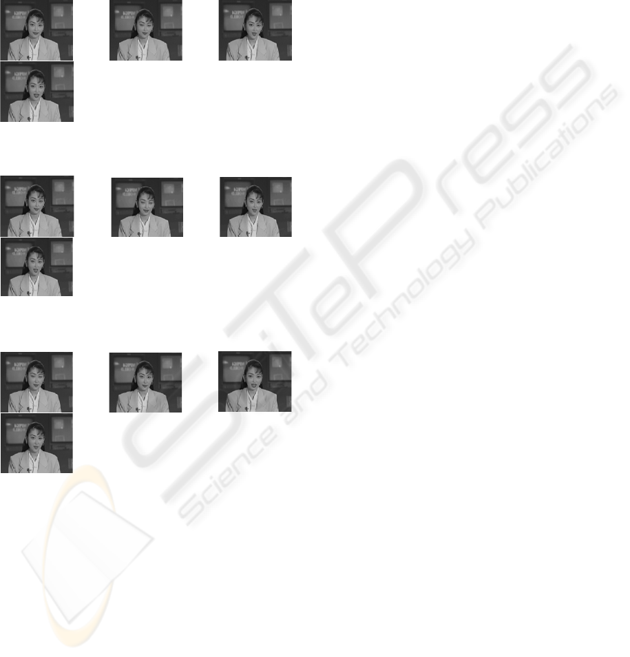
Figures 5(a) shows the original images from the
“Akiyo” video sequences at frames 1, 5, 8, 10, 12
and 16. Figures 5(b) and 5(c) below shows selected
frames (frames 1, 5, 8, 10, 12 and
4 CONCLUSION AN
SUGGESTIONS
decompressed images from the
sequences using the first 16 fram
wavelet decompositions and
fitting on both previous and proposed method
As for the findings and analyses, the range of
PSNR acquired using the first 16 frames results the
uppermost value of
PSNR seeing that lesser points
will have lesser deviation as far as accuracy is
concerned. Using 32 frames may grant a sensibly
reduced file size with a reasonable compression
ratio, but a massive concession on the image quality
has to be acknowledged. Nonetheless, engaging 16
frames distributes the most rationale results with a
balanced trade-off as far as efficiency and quality is
concerned. On average, using
50=p
appears to
have a higher
PSNR but the compromise in file size
is too massive.
Regardless of the method used, the highest value
of
PSNR is obtained when fewer frames are
considered. Even so, the desired option will be the
one with a good trade-off between the file size and
the
PSNR as they have a vast imp the storage
efficiency and the image quality respectively. The
proposed method of polynomial fitting applied to the
wavelet coefficients of the relevant pixels produced
a f ne outcome with anticipated level of efficiency as
far as compression is concerned.
Nonetheless, there exist certain limitations to this
conversed method where it is only more suitable for
video sequences with minimal motions and minor
changes in the background. Example of such
application is the storage of surveillance camera
footage or a closed-circuit television. This study is
still in the ground work and has heaps of rooms for
incessant advancement and enhancem
VISAPP 2009 - International Conference on Computer Vision Theory and Applications
164
res
e
ames 1, 8, 12 and 16 using the
ent method at p=25.
RE
SCAS’06, Vol. 2, 128-
Duanmu, C. J., 2006. Fast Scheme for the Four-step
Dunn, J.R., 2002. Faster Smarter Digital Video, Microsoft
Kap
Series Information,
Ko
Singapore:
Lia
ression. IEEE Trans. on Image
Lin . M., 2004. Wavelet Video Coding
its and Systems for Video Technology, Vol. 14,
Sym
Tau 2000:
Image Compression Fundamentals, Standards and
Practice, Kluwer Academic Publishers.
Zadeh, P.B., Buggy, T., Akbari, A.S., 2008. Statistical,
DCT and Vector Quantization-based Video Codec.
IET Image Processing, Vol. 2, Issue 3, 107-115.
olving a suitable level of wavelet and identifying
an appropriate degree of polynomial along with
suitable polynomials for different pixels throughout
the frames may be considered. Also, development of
a model to obtain the optimal
p for any domain of
dataset can be deemed. Color video sequence can
also be given a thought.
Figure 5(
first 16 frames o
a): Images of th
f the Akiyo v
e frames 1, 8, 12
ideo sequences.
and 16 using th
Figure 5(b): Images of frames 1, 8, 12 and 16 using the
first 16 frames using the previous method.
Figure 5(c): Images of fr
first 16 frames using the curr
FERENCES
Averbuch, A., Lazar, D. and Israeli, M., 1996. Image
Compression Using Wavelet Transform and
Multiresolution Decomposition. IEEE Trans. on
Image Processing, Vol. 5, Issue 1, 4 –15.
T.Nithyaletchumy Devi, Lim W.K., Tan Y.F., Tan W.N.,
Teng, H.T. and Chang, Y.F., 2008. Video
Compression Using Temporal Polynomial Fitting on
Wavelet Coefficients. 16
th
Int. Symposium of Science
and Mathematics (SKSM).
Duanmu, C. J., 2006. Fast Scheme for the Thee-step
Search Algorithm by the Utilization of Eight-bit
Partial Sums. 49
th
IEEE Int Midwest Symposium on
Circuits and Systems. In MW
131.
Search Algorithm in Video Coding. IEEE Int
Conference on Systems, Man and Cybernetics. In
SMC’06, Vol. 4, 3181-3185.
Press.
lan, I., 2004. Applying the Haar Wavelet Transform to
Time
http://www.bearcave.com/misl/misl_tech/wavelets/haa
r.html
ornwinder, T.H., 1993. Wavelets: An Elementary
Treatment of Theory and Applications,
World Scientific.
ng, J., Tu, C., Tran, T. D., 2005. Optimal Block
Boundary Pre/Postfiltering for Wavelet-based Image
and Video Comp
Processing, Vol. 14, Issue 12, 2151-2158.
, K. K., Gray, R
With Dependent Optimization. IEEE Trans. on
Circu
Issue 4, 542-553.
es, P.D., 2001. Video Compression Demystified,
McGraw Hill.
Symes, P.D., 2003. Digital Video Compression, McGraw
Hill.
bman, D.S., Marcellin, M.W., 2002. JPEG
TEMPORAL VIDEO COMPRESSION USING MODE FACTOR AND POLYNOMIAL FITTING ON WAVELET
COEFFICIENTS
165
