
PHOTO REPAIR AND 3D STRUCTURE
FROM FLATBED SCANNERS
Ruggero Pintus
CRS4 (Center for Advanced Studies, Research and Development in Sardinia), Parco Scientifico e Tecnologico, POLARIS
Edificio 1, 09010 Pula (CA), Italy
Thomas Malzbender
Hewlett-Packard Laboratories, 1501 Page Mill Road, Palo Alto, CA 94304, U.S.A.
Oliver Wang
University of California, Santa Cruz, 1156 High Street, Santa Cruz, CA 95064, U.S.A.
Ruth Bergman, Hila Nachlieli, Gitit Ruckenstein
Hewlett-Packard Laboratories, Technion City, Haifa 32000, Israel
Keywords: Scanners, 3D reconstruction, Photo repair, Photometric stereo.
Abstract: We introduce a technique that allows 3D information to be captured from a conventional flatbed scanner.
The technique requires no hardware modification and allows untrained users to easily capture 3D datasets.
Once captured, these datasets can be used for interactive relighting and enhancement of surface detail on
physical objects. We have also found that the method can be used to scan and repair damaged photographs.
Since the only 3D structure on these photographs will typically be surface tears and creases, our method
provides an accurate procedure for automatically detecting these flaws without any user intervention. Once
detected, automatic techniques, such as infilling and texture synthesis, can be leveraged to seamlessly repair
such damaged areas. We first present a method that is able to repair damaged photographs with minimal
user interaction and then show how we can achieve similar results using a fully automatic process.
1 INTRODUCTION
Flatbed scanners are commonly available, low cost,
and commercially mature products that allow users
to digitize documents and photographs efficiently.
Recently, flatbed scanner products that incorporate
two separate and independently controlled
illumination bulbs have become available (HP,
2007). The original intent of such a two bulb design
is to improve color fidelity by illuminating the
document or photograph with separate chromatic
spectra, effectively making a 6 channel measurement
of color instead of the conventional 3 channel
measurement, improving color fidelity. We
demonstrate that such hardware can also be used to
estimate geometric information, namely surface
normals, by a novel approach to photometric stereo.
These extracted surface normals can be used in
several ways. Scanned objects can be relit
interactively, effectively conveying a sense of 3D
shape. Normal information can also be used to
automatically repair damaged surfaces of old
photographs. We have found that tears and creases
in old photographs can be reliably detected since
they are associated with surface normals that are not
strictly perpendicular to the surface of the scanner
plate. Once detected, these imperfect pixels can be
replaced by leveraging infilling and texture synthesis
methods, effectively repairing the print in an
automatic manner. Although products do exist on
the market that specialize in recovery of 3D
information from physical objects, these are 2-4
40
Pintus R., Malzbender T., Wang O., Bergman R., Nachlieli H. and Ruckenstein G. (2009).
PHOTO REPAIR AND 3D STRUCTURE FROM FLATBED SCANNERS .
In Proceedings of the Fourth International Conference on Computer Vision Theory and Applications, pages 40-50
DOI: 10.5220/0001789500400050
Copyright
c
SciTePress

orders of magnitude more expensive than
commercial flatbed scanners and involve significant
mechanical complexity. Our method requires no
hardware modification to current products, no
additional user interaction, and can scan objects in a
very short amount of time.
Section 2 provides an overview of related work.
Section 3 presents the entire procedure used to
estimate the surface gradient from a flatbed scanner
with two bulbs. Sections 4 and 5 describe the
photograph repair application and the automatic
process to remove tears and creases. Two methods
are presented, one that works on two pairs of images
with an intermediate manual rotation, and another
method that achieves fully automatic repair from a
single pair of images. Section 6 summarizes other
applications and Section 7 provides paper summary
and conclusions.
2 RELATED WORK
In this paper, we use principles from photometric
stereo to recover per-pixel surface normals of a 3D
object or photograph. The recent introduction of
flatbed scanners that employ 2 separately controlled
light sources greatly facilitates this approach (fig.2).
As an alternative approach to gathering 3D structure
from flatbed scanners, (Schubert, 2000)
demonstrates how they can be used to collect
stereoscopic images. Although no explicit extraction
of depth or 3D information is performed, a good
percept of 3D shape can be achieved with this
approach. Schubert leverages the fact that in such
CCD-based scanners, the resulting scanned images
perform a orthographic projection in the direction of
the carriage movement, y, but a perspective
projection in the orthogonal direction, x. By
repositioning the object with variation in the x
placement, views of the object from multiple
perspectives are achieved. Stereograms can be
produced to good effect by arranging and viewing
these images appropriately.
Although the hardware prototype has
significantly more complexity than a flatbed
scanner, (Gardner et al., 2003) shows an elegant
approach using Lego Mindstorm and linear light
sources to collect normal and albedo information,
along with higher-order reflectance properties. This
approach can not be leveraged on today’s flatbed
scanners due to the fixed geometric relationship
between the light sources and imagers in
conventional scanners. A related, unpublished
approach was independently developed by (Chantler
and Spence, 2004). Their acquisition methodology is
similar, and also discusses the approach of
simultaneously performing registration and
photometric stereo. However, applications such as
photo repair and reflectance transformation are not
pursued. (Brown et. al, 2008) describe an approach
for digitizing geometry, normals and albedo of wall
painting fragments using the combination of a 3D
scanner and a conventional flatbed scanner. Surface
normals are acquired with a flatbed scanner by
combining 2D scans. They demonstrate the
improved normal fidelity that can be achieved by
photometric stereo as opposed to 3D scanning.
Our image repair application is motivated by
earlier work on removing dust and scratch from
scanned images. (Bergman et al., 2007) describe a
range of solutions for dust and scratch removal. For
scans of transparent media, i.e. negative or slides,
(DIGITAL ICE, 2001) introduced the use of Infra-
red (IR) hardware. The IR light is blocked by dust
and scattered by scratches, thereby enabling very
accurate defect detection. For prints, detection is
based upon characteristics of the defects in the
digital image, e.g., defects that are light and narrow.
While this approach correctly identifies defects,
it is prone to false detection of image features with
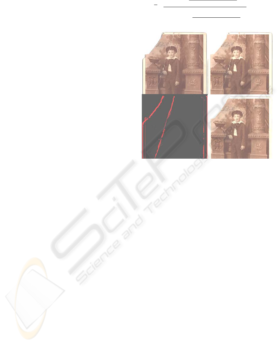
Figure 1: Left: Original scan of a damaged photograph. Middle: 3D structure present on the surface of the print extracte
d
by our method. Right: Automatically repaired photograph using 3D structure information and infilling methods.
PHOTO REPAIR AND 3D STRUCTURE
FROM FLATBED SCANNERS
41
similar characteristics. We propose a detection
method for scanned prints based on 3D surface
normals.
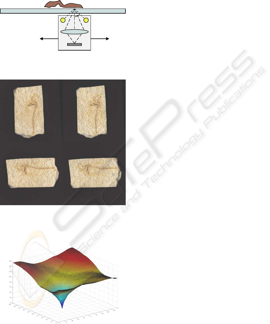
Scanner Platen
CCD
Bulbs
Optics
Scanned Object
Lighting and Imaging
Assembly Translates
α
Figure 2: Typical flatbed scanner – side view. Note the
lighting assembly moves with the imager, effectively
providing two lighting directions across the entire scan.
Figure 3: Images captured by our modified HP Scanjet
4890. Pairs of scans are captured with only one of two
bulbs actuated independently. For the second pair, the user
has manually rotated the fossil by roughly 90 degrees.
This effectively yields 4 lighting directions.
Figure 4: Prediction error for the fossil shown in Fig. 2
using the SIRPH algorithm. X: rotation, Y: translation in
y, Z: error.
3 NORMAL CAPTURE
FROM FOUR IMAGES
Given at least 3 images of a surface taken with
different lighting directions, it is possible to recover
per-pixel estimates of surface normals and albedo
using photometric stereo. Flatbed scanners currently
capture a single image under static lighting
conditions, but they often employ 2 bulbs to
illuminate the subject. These two bulbs provide
illumination from either side of the scan line being
imaged. If we independently control these 2 bulbs,
the scanner is capable of taking 2 scans, effectively
one with lighting from above, and another with
lighting from below. We have experimented with
two hardware platforms that allow such scans to be
acquired. First, we modified an HP Scanjet 4890 to
allow us to manually activate each of the two bulbs
separately. Later, when the HP ScanJet G4050
became available with separate control of each bulb
supported in software, we switched to this platform.
Both platforms provide 2 images with different
lighting. For the first approach we describe, we
retrieve another pair of images under new lighting
directions by prompting the user to manually rotate
the object they are scanning by roughly 90 degrees.
At this point, two new scans are taken, again with
each bulb activated independently yielding 4 images
of the object with 4 different light source direction
(fig.3). However, the two sets of images are not
registered relative to each other, so we have
introduced a difficult registration problem since the
images are all taken under varying lighting
directions. We have developed a method to robustly
solve this registration problem called SIRPH, which
stands for SImultaneous Registration and
PHotometric stereo.
In section 4.2 we present a method that avoids
any approximate manual rotation and works directly
with just 2 images.
SIRPH exactly solves for the two translation and
one rotation parameters, (x,y,θ), that are introduced
by the user rotating the object by roughly 90
degrees. At the same time, it solves for the surface
orientation (normals) at each pixel. The SIRPH
method initializes the rotation and translation
parameters, then uses photometric stereo (Barsky et
al., 2003) on three of the images to compute surface
albedo and normals per pixels. Two of the images
used are from one set of scans and a third is taken
from the other set which is rotated and translated
according to the current best guess of the rotation
and translation parameters. Photometric stereo gives
us an estimation of normals and albedo of the
VISAPP 2009 - International Conference on Computer Vision Theory and Applications
42

scanned object, which can be used to estimate the 4
th
image by the Lambertian reflectance model:
)( LNI
•
=
′
ρ
(1)
where
ρ
is surface albedo, N is normal vector and
L
is the vector pointing to the light source. The
estimated image, I’, is then compared to the actual
4
th
image, I
4,
giving us a prediction error (fig.4) for
parameters (x,y,θ) as follows:
∑
⊂
−
′
=
Pp
ppprediciton
IIE
24
)(
(2)
where P is the set of all pixels in an image, and I
p
corresponds to the pth pixel in image I.
Fortunately, this prediction error is typically well
behaved, and iterative nonlinear optimization
techniques can be employed to find the well defined
minimum. After experimenting with several
nonlinear optimization methods, namely Levenberg-
Marquart, Gauss-Newton and Simplex, we finally
settled on a simple hierarchical approach that was
both robust and fast. In our technique, we perform
an iterative search starting at a low resolution
working up to the original size image. At each
resolution level, samples are taken at the current
position and at a +/- step size increment in each of
the 3 dimensions of our search space. The lowest
error of these 8 + 1 sample points is chosen as the
base for the next iteration. If the same base point is
chosen, the step size is halved and further iterations
are taken. Once the step size is below a threshold,
convergence is achieved and we start the search at
the next resolution level with the current
convergence state. At each level, this technique is
commonly known as compass-search.
Because compass-search can get stuck in local
minima, a good starting point is key to convergence.
We therefore perform the entire search multiple
times at the lowest resolution, each “seeded” with a
different starting point. Because the optimization
occurs very quickly at low resolution, we are able to
use many different starting points that cover a large
area of the sample space. We then take the best
match from all these to start the search at the next
level. After we converge on the original resolution
image, we will have robustly recovered the required
translation and rotation parameters to register the 2
pairs of images, as well as a surface normal per
pixel. We tested this method on a variety of objects
and notice that it is capable of achieving correct
convergence in almost all cases, including very
difficult ones such as circular objects with low
amounts of texture.
4 PHOTOGRAPH REPAIR
APPLICATION
We have outlined our procedure for extracting 3D
normals and albedo from objects using a flatbed
scanner. We now present several applications of this
method, the most significant being the automatic
detection and repair of creases and tears in scanned
photographs. Almost everyone has a one of a kind
photo of their child, parent or grandparent that has
been battered over the years. Old photographs often
have tears, creases, stains, scratches and dust.
Fortunately, the technology to restore such images
exists today through a variety of digital imaging
tools. Your local photo-finishing lab can do it for a
fee. It can also be done in the home using a scanner,
printer and photo editor such as Adobe Photoshop.
This path to photo restoration is fairly tedious and
requires some expertise in the use of the photo
editor.
Although a reliable capability exists already to
detect and repair defects in transparencies such as
dust and scratches (using IR illumination), no such
robust counterpart exists for the detection and repair
of damaged prints. Infilling techniques from the
transparency domain can be leveraged for the repair
process, but the robust detection of damaged regions
of a print is lacking. Our method provides such a
capability, since the damage one that is looking for
is associated with 3D perturbations. Figure 1 shows
one example of this capability that we have
prototyped with a HP 4890 scanner. The next two
sections describe the procedures used for this
application. We first present the 4 image procedure,
which has the drawback that it requires the user to
rotate the photograph. In section 4.2 we introduce a
2 image process that performs the same task, but
without any user intervention.
4.1 Defect Maps from Normals
The 3D normals give a general indication of the
location of the defects in the scans. In principle, high
normal perturbations from the z axis (defined to be
pointing up from the photograph) indicate a defect,
and low normal perturbations indicate undamaged
portions of the print. However, simply taking a
threshold of such perturbations produces a defect
map with insufficient accuracy.
This map may miss portions of the defect, e.g., very
fine portions of a crease, and it is likely to have
some false detections, e.g., the red pixels near the
boy’s left sleeve in Figure 5 (left). To overcome
these issues, we use a two step approach. We first
PHOTO REPAIR AND 3D STRUCTURE
FROM FLATBED SCANNERS
43

Figure 5: Constructing defect maps using the 4-image
procedure. Left: Expansion labeling computed from the
normals. Right: Refinement detection map for light
defects.
expand the set of candidate pixels, along features
such as creases, then apply a refinement stage on the
expanded mask to select a subset of these pixels that
will need repair. The expansion phase thresholds the
3D normal information at two levels. Pixels with
very high normal perturbations are marked as
defective. Pixels with less high normal perturbations
are marked as candidates. A voting algorithm,
closely related to (Medioni, 2000), extends the
defects. Connected components of the marked pixels
are computed. Each component exerts a field of
influence based on its shape and size. For example, a
crease extends a field in the direction of the crease.
The fields of influence from all the components are
added for an overall vote at each pixel. Defective
pixels are marked pixels with high votes and
unmarked, connected pixels with very high votes.
The purpose of the refinement step is to select a
subset of pixels identified in the expansion phase as
the final selection that will require repair. The
refinement step uses a grayscale representation of
the image and creates a smoothed reference image
that does not contain the defects by applying a
median filter. Defective pixels can either be too light
or too dark. In both cases the difference between the
grayscale representation and the reference image is
significant for defective pixels. Thresholding the
difference image is prone to detection of some small,
bright image features, hence we label pixels as
defective only if they are both in the expanded set of
candidate pixels and yield a big difference between
the grayscale and reference images. We further
refine the defect map by detecting the contour of the
defect using classification. Looking at a
neighborhood near a defect we have gray-level data
and a label for each pixel of clean, defect-light or
defect-dark. We label several pixels around the
contour of the defect as unknown and classify them
using Quadratic Discriminant Analysis (Hastie et al.,
2001). Without contour classification, a trace of the
tear would remain after repair.
This refinement step is repeated once for light
defects and again for dark defects. From a normal
viewing distance the white areas are the most
striking defect. A closer look usually reveals dark
shadows adjacent to the white tear. Indeed, if we
only repair the white defects, we are left with an
apparent crease in the image due to the shadowed
pixels. We obtained the best results by detecting and
repairing (infilling) light defects and then detecting
and repairing dark defects.
4.2 Normal Components from Two
Images
The 4-image procedure has the drawback that the
user must rotate the photograph to compute normals
(or both surface derivatives along x and y). It is well
known that photometric stereo requires at least three
images for a complete gradient computation (Barsky
et al., 2003). We have developed a method to use
two images to estimate one component of the
derivative (in our case the derivative along y, i.e.
along image columns). In this way, we avoid
needing the user to rotate the sample manually.
However, we encounter two limitations. First, we
have less information to detect defects, and second,
the algorithm can’t recover tears and creases that are
precisely aligned with the image columns. We can
address the first issue with a more complex
procedure. To avoid perfectly vertical defects, we
recommend that the user reorient the photo in the
scanner.
An unmodified, commercial HP ScanJet G4050
scanner, which we used for these experiments,
introduces the further complication that the
chromatic spectra of each bulb is intentionally
designed to be different. As mentioned, this was
done to improve color fidelity effectively making a 6
channel measurement of color. This chromatic
difference is problematic for photometric stereo. We
overcome this issue by recovering 2 separate 3x1
color transform matrices that map each image into a
similar one dimensional ‘intensity’ space, in which
we perform photometric stereo computations. These
color transform matrices have been derived by
scanning a Macbeth color chart exposed with each
bulb independently, and then minimizing the
difference in transformed response.
A second problem with flatbed scanners is that
the mechanical repeatability of the scan mechanism
is not perfect, causing slight vertical misalignment
between the pair of scans. To correct this we
VISAPP 2009 - International Conference on Computer Vision Theory and Applications
44
upsample each scanned image in the vertical
direction, and then we find the misalignment by
minimizing the integral of the surface gradient in y
direction.
We approximate the lighting geometry with
lighting direction vectors
[]
[]
⎩
⎨
⎧
=
=
222222
111111
cossinsincossin
cossinsincossin
αβαβα
αβαβα
l
l
(3)
with
⎪
⎪
⎪
⎩
⎪
⎪
⎪
⎨
⎧
−=
+=
===
2
2
6
2
1
21
π
β
π
β
π
ααα
(4)
Using the Lambertian reflectance map (Horn,
1986) we obtain
()
⎪
⎪
⎩
⎪
⎪
⎨
⎧
++
+
==
++
+−
==
22
022
22
011
1
cossin
1
cossin
,
qp
q
LRI
qp
q
LqpRI
αα
ρ
αα
ρ
(5)
where I1 and I2 are the images, p and q are surface
derivative along x and y respectively, L0 is the light
source magnitude and ρ is the surface albedo.
Solving for q, we obtain:
()
()()
()()
yxIyxI
yxIyxI
yxq
,,
,,
tan
1
,
12
12
+
−
=
α
(6)
In this way, we can recover the surface
derivative value in one direction. Note that although
this derivative along y is exactly recovered, the
estimation of the other component of the surface
gradient with just a pair of images is not possible
without making some assumption on p, such as
convexity or smoothness assumptions.
To solve for the misalignment, we assume, for
now, that most of our scanned photograph is flat
(q=0). We find the best alignment minimizing the
function
∑∑
∑∑
==
Δ+Δ+
Δ+Δ+
==
+
−
=
=
N
i
M
j
ji
us
jjii
us
ji
us
jjii
us
N
i
M
j
us
ji
II
II
q
11
,
1
,
2
,
1
,
2
11
,
tan
1
α
(7)
where
us
I
2,1
and
us
q are the gray level upsampled
images and scanned surface derivative along y,
(Δi,Δj) is the misalignment and N and M are
respectively the number of rows and columns. We
used upsampled images to compute subpixel
misalignments. After correcting the misalignment,
we downsample images to their original resolution.
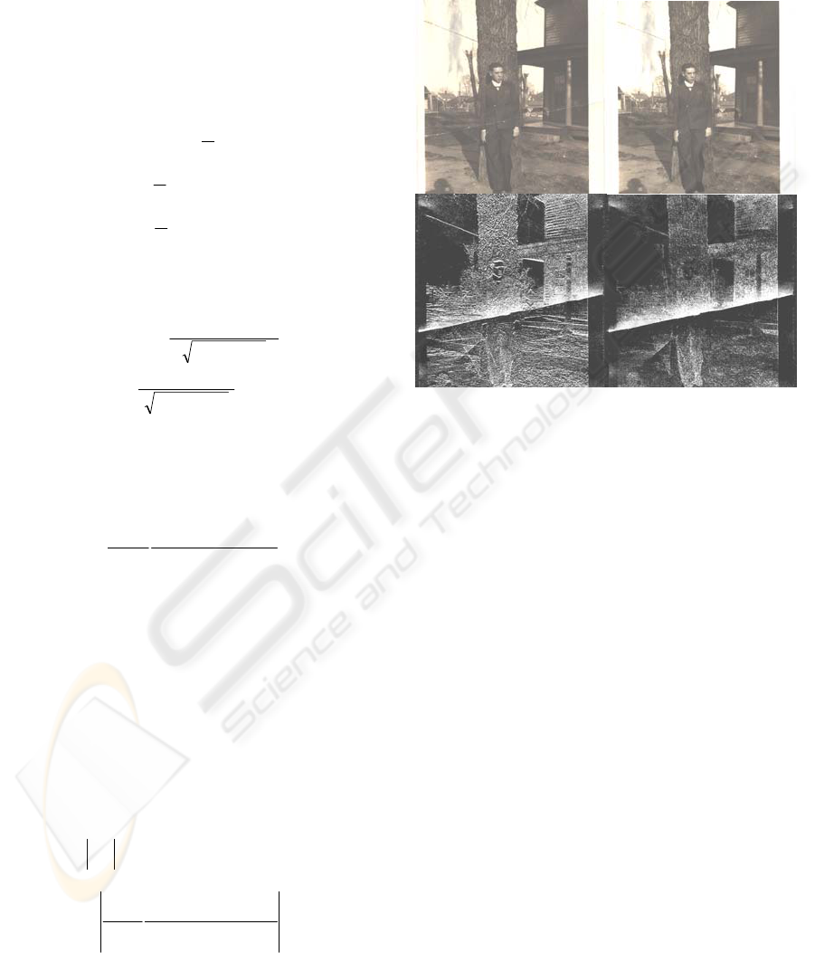
Figure 6: UL: Scanned image. UR: Repaired image. LL:
Absolute value of the y derivative before the alignment
step. LR: After alignment.
Fig.6 shows the derivative along y before and
after the alignment step. We can see, in Fig. 6 LL,
that there are some image edges that should not be in
an albedo independent signal (such as the surface
gradient), while such image content dramatically
decreases after the images are aligned as shown in
Fig. 6, right.
After the color transformation and alignment
operations, these two source images can be used as
input to compute a defect map that will indicate
where tears and creases on the surface of the
photograph are present. Unfortunately, the q image
recovered at this point suffers from numerical noise
in regions where the colors are dark (fall near the
origin if the RGB color cube). Fig. 7 shows how the
darkest square is noisier than the others, while the
brightest gray one on the bottom right is practically
invisible. Recall that our goal (regarding the
repairing task) is to differentiate pixels associated
with tears and creases from flat regions of the
photograph, not necessarily to recover exact
estimates of the gradient component. To this end, we
have found it useful to combine the gradient and
color difference information to define a composite
image which is the normalized version of the
product of the color differences multiplied by the
PHOTO REPAIR AND 3D STRUCTURE
FROM FLATBED SCANNERS
45
()
(
)
()
[]
yxm
yxm
yxm
,max
,
,
ˆ
=
(8)
estimated vertical derivative:
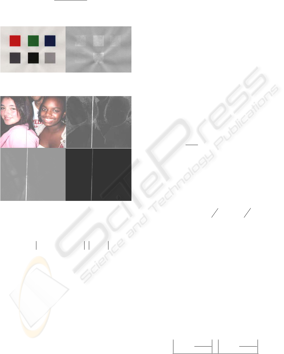
Figure 7: Left: Scanned image; Right: Recovered gradient
component along y.
Figure 8: UL: Scanned image. UR: Gradient component
absolute value along x. LL: Absolute value of the
difference between the two acquired images. LR: Mask
),(
ˆ
yxm
is the input of the defect trimap generation step.
() ()()()
yxqyxIyxIyxm ,,,,
12
⋅−=
(9)
The gray level difference image has a value near
zero where q is near zero and doesn’t contain
numerical errors due to the albedo. This feature is
useful to eliminate the numerical errors in q, even if
it adds some albedo dependent signal in regions
containing defects. Note that we could still have a
problem if a defect pixel has dark albedo. In practice
we find that for these pixels, even if the (I
1
,I
2
) vector
has a low magnitude, the difference of its
components is big enough to distinguish the defect.
In Fig.8 we can compare the gradient and difference
images. While the noise in the gradient image is
evident (we can distinguish the outline of the faces),
the difference image has almost no numerical noise.
Note that the defective pixels are also less visible in
the difference image, but are enhanced in the
composite image, m, due to the strong signal in the
gradient. In short, we have used the gradient to
enhance the signal in defect regions and use the
difference image to avoid noise in the flat zones.
Note that in figure 8 we display the scanned images
rotated 90 degrees for clarity, effectively placing the
light sources to the left and right in the figure.
Fig.8 LR shows the mask
()
yxm ,
ˆ
computed
from the source images. This obtained mask has
gray level values that must be thresholded in some
way to decide how high the value must be to identify
a defect pixel. A single threshold across all photos
fails to be adequately robust. To this end, we define
a function
m
~
:
()
()
()
⎩
⎨
⎧
≥→
<→
=
γ
γ
γ
yxm
yxm
yxm
,
ˆ
1
,
ˆ
0
,,
~
(10)
This function is simply a binary image, with γ as
threshold. The percentage of the image lying above
this threshold is simply
() ()
∫∫
= dxdyyxm
NM
A
γγ
,,
~
1
(11)
where N and M are respectively rows and columns
number.
We compute a trimap by classifying each pixel
as being either ‘defect’, ‘uncertain’ or ‘non-defect’.
We choose the 2 thresholds for this classification by
finding the knee in the relationship between A and γ.
Specifically, we set two thresholds on the angle the
curve makes, namely
8
π
−
and
8
3
π
−
which are
25% and 75% respectively of the angular range. A
concrete example may clarify this approach. Fig.9
shows the function
(
)
γ
A
for the sample in fig.8.
This is a display of the image area as a function of
threshold γ. Choosing the angle thresholds above
corresponds to γ thresholds of 0.005 and 0.0094 for
constructing the tri-map. Fig.10 shows the trimap in
which red pixels are defect, bright grey pixels are
non-defect and black pixels are the unknown ones.
In this example the defects are fairly easy to detect
yielding a small number of unknown pixels.
Once such a trimap is constructed we need to
classify the unknown pixels. For this we use
Quadratic Discriminant Analysis (QDA) (Hastie et
al., 2001). As features we use the q and difference
images as well as the following image:
()
()
(
)
()
()
2
cos
,
,
cos
,
,
,
21
α
ρ
α
ρ
yxE
yx
yxE
yx
yxf
−+−
=
(12)
VISAPP 2009 - International Conference on Computer Vision Theory and Applications
46
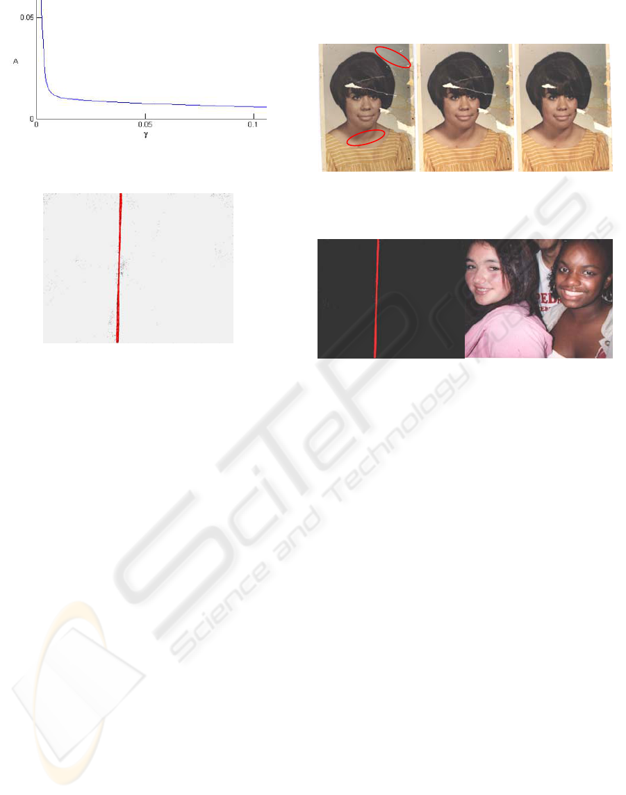
Figure 9: The function
()
γ
A
for Fig. 8a.
Figure 10: The trimap for Fig. 8a: red pixels are defect,
light grey are non-defect and black are unknown (appear
sparse and small in this case).
This equation is derived from eq. 5 by setting L
0
to 1 and p(x,y)=0. After normalizing, f(x,y) has low
values in the non-defect pixels and high values
(albedo dependent) in the defect pixels. Note that we
have computed the albedo using classical
photometric stereo methods and assuming p=0.
Although in practice the unknown p does not always
equal zero, especially for defective pixels, this
assumption still yields the function, f(x,y), which is
useful in distinguishing defect from non-defect
pixels.
We apply QDA, trained on the known defect and
non-defect pixels, and applied to the unknown
pixels, for each photograph independently. This
yields a labeling of all pixels as being either
defective or not, which along with the albedo image,
is processed by the refinement step, as described in
4.1. We use the albedo instead of one of the original
images because some low frequency creases are
removed by simply computing the albedo, even
when they are present in the source images, as
shown in Figure 11. We also apply the infilling
procedure to the albedo image, not one of the
original source images, since the albedo image is not
prone to darkening introduced by the interaction of
the non-perpendicular lights and subtle low
frequency curvature on the surface of the
photograph. Fig.12 shows the automatically detected
defect map, which is the input for the refinement
step and the repaired image after the infilling
algorithm.
Figure 11: Subtle, low frequency creases are avoided in
the albedo image. Left: Scanned image. Middle:
Recovered albedo. Right: repaired image.
Figure 12: Left: Defect map before refinement step. Right:
Repaired image after infilling algorithm.
Methods do exist in the literature that attempt to
compute all gradient information from two images
(Onn et al., 1990) (Tu et al., 2003) (Yang et al.,
1992) (Petrovic et al., 2001). Unfortunately, after
prototyping several of these, we find them
insufficiently robust in practice.
5 INFILLING ALGORITHMS
The input to the infilling algorithm is a digital image
in which every pixel is classified as either defective
or non-defective. The non-defective pixels can be
further classified as candidates or non-candidates for
replication. A data structure is provided in which
defective pixels are arranged in connected
components.
Our algorithm essentially replaces every
defective pixel by a value computed from selected
candidate pixels. A candidate pixel may be any non-
defective pixel of the image. The selection is based
on (1) the spatial distance between the defect
location and the candidate location and (2) the
similarity of pixel values in the local neighborhoods
of the two pixels. Two parameters govern the
selection: the width W of a square region around the
defect in which candidates are examined and the
width w of a square local neighborhood surrounding
PHOTO REPAIR AND 3D STRUCTURE
FROM FLATBED SCANNERS
47
and including a pixel. Typically, the region width W
is much greater than the neighborhood width w. For
example, we used a region of 200×200 pixels and
neighborhoods of 7×7, 9×9, and 11×11 pixels.
As a pre-processing step, we compute texture
descriptors of all the local neighborhoods of
candidate pixels in the image. In our
implementation, we used mean and standard
deviation of values in a surrounding w×w
neighborhood as texture descriptors. The
computations are done once for every candidate
pixel and do not depend on any defective context.
Pixel reconstruction is done for groups of connected
components sequentially. The recommended order
of pixel reconstruction within a single connected
component is from the outside in. This order of
computation creates fewer image artifacts. To
reconstruct a defective pixel, we examine its
surrounding w×w neighborhood while ignoring
defective pixels in that neighborhood. The texture
measures of the local neighborhood are computed,
namely the mean and standard deviation of the non-
defective pixel values. We then find 10% of the
candidates in the W×W region around the defect
whose texture measures best match the texture
measures of the target neighborhood. To accelerate
the search for the best 10% of all candidates, we use
an efficient data structure where all the candidates in
a region are sorted by both the mean and the
standard deviation of their surrounding w×w
neighborhoods.
For each of the 10% of selected candidate pixels,
we further compare its w×w neighborhood relative
to the defective pixel and its neighborhood.
Neighborhoods are compared by the sum of squared
differences (SSD) of respective values. Two
approaches were used to compute the output pixel
value, resulting in two different algorithms. The first
approach, which is based on (Efros and Leung,
1999), takes the best pixel, i.e. lowest SSD. The
second approach computes a weighted average of all
the candidates, where the weighting is based on the
SSD measure as follows. Let Q = q
1
,q
2
,…,q
w·w
be
the two dimensional neighborhood surrounding the
pixel to repair and let C be the set of candidate
neighborhoods. For a neighborhood P in C, we use
the notation P = p
1
,p
2
…,p
w·w
and denote its central
pixel by p. Let G=g
1
,g
2
…, g
w·w
be a Gaussian spatial
filter, and let h be a real value weight filter. For a
defective pixel i in the neighborhood P, the
corresponding value of the Gaussian filter g
i
is set to
0. The new value for the pixel is:
∑
∑
∑
∑
∈
⋅
=
∈
⋅
=
−⋅−
⋅
−⋅−
=
Cp
ww
i
iii
Cp
ww
i
iii
h
qpg
p
h
qpg
q
)
)(
exp(
)
)(
exp(
2
0
2
2
0
2
(13)
Figure 13: UL: scanned image. UR: albedo. LL:
automatically computed defect map before refinement.
LR: repaired image using infilling algorithms.
This method is adapted from the NL-Means
denoising algorithm (Buades et al., 2005). By
applying SSD comparisons to only 10% of the
candidate neighborhoods instead of all the
neighborhoods in the surrounding region, we attain
approximately a factor of ten speed up, and no
visible degradation in image quality. This speed up
makes these algorithms applicable in practical
infilling tasks, as those described in subsequent
sections.
Note that the accelerated infilling algorithms are
still slower than simple local operations such as
median filtering or averaging. These local
algorithms however tend to blur image details, so
they are not acceptable for a photo repair
application. Fig.13 shows the entire automatic
procedure (using two images, the automatic defect
detection, the refinement procedure and the infilling
algorithm) for the photograph in fig.1.
6 ADDITIONAL APPLICATIONS
In addition to allowing the repair of old photographs,
the combination of color and normal or reflectance
data taken from physical objects can be applied in
VISAPP 2009 - International Conference on Computer Vision Theory and Applications
48
other ways. Transforming reflectance data based on
normal information to enhance surface perception of
detail has already been demonstrated (Malzbender et
al., 2001), (Toler-Franklin et al., 2007), (Freeth et
al., 2006). A further example on data captured by
our flatbed scanner is shown in fig. 14. Combing
multiple images taken under multiple lighting in a
spatially varying manner can also yield enhanced
visualizations (Fattal et al., 2007). Data captured
from our scanners can also be used for these
methods. Lastly, normal information from
photometric stereo can of course be integrated to
recover a 3D model of surface structure (Horn,
1986). This geometry will typically suffer from a
number of artifacts, such as low-frequency warping
from the integration of inaccuracies and mishandling
of discontinuities in the object geometry.
7 CONCLUSIONS
We have presented a technique to recover the 3D
normal structure of an object using a conventional
flatbed scanner. This allows relighting, and limited
geometry capture. We have also demonstrated an
application to the automatic repair of damaged
photographs exhibiting creases or tears. Although
we prototyped this functionality on a particular HP
scanner, the approach is applicable to any flatbed
scanner that uses 2 bulbs to illuminate the platen,
which is the common case.
Outstanding challenges still remain. First, the
depth of geometry we can handle is limited by the
optics of the scanner. For the unmodified scanners
we used in our work, we measured this to be
approximately 1 cm. Second, a geometric warp must
be applied to the raw scanner data to rectify the
images before registration. This must be done to
sub-pixel accuracy to obtain reliable normal
estimates. Also, a limitation of the 2 image approach
we have taken (but not our 4 image approach) is our
inability to detect perfectly aligned defects. This can
however be accommodated in most cases by the user
simply avoiding such defects with a rotation of the
photograph to re-align it.
We have investigated techniques in the literature
that attempt to recover both surface derivatives
components, (p,q), from a single pair of images, but
have found them insufficiently robust. In future
work, we would like to develop such a robust
method.
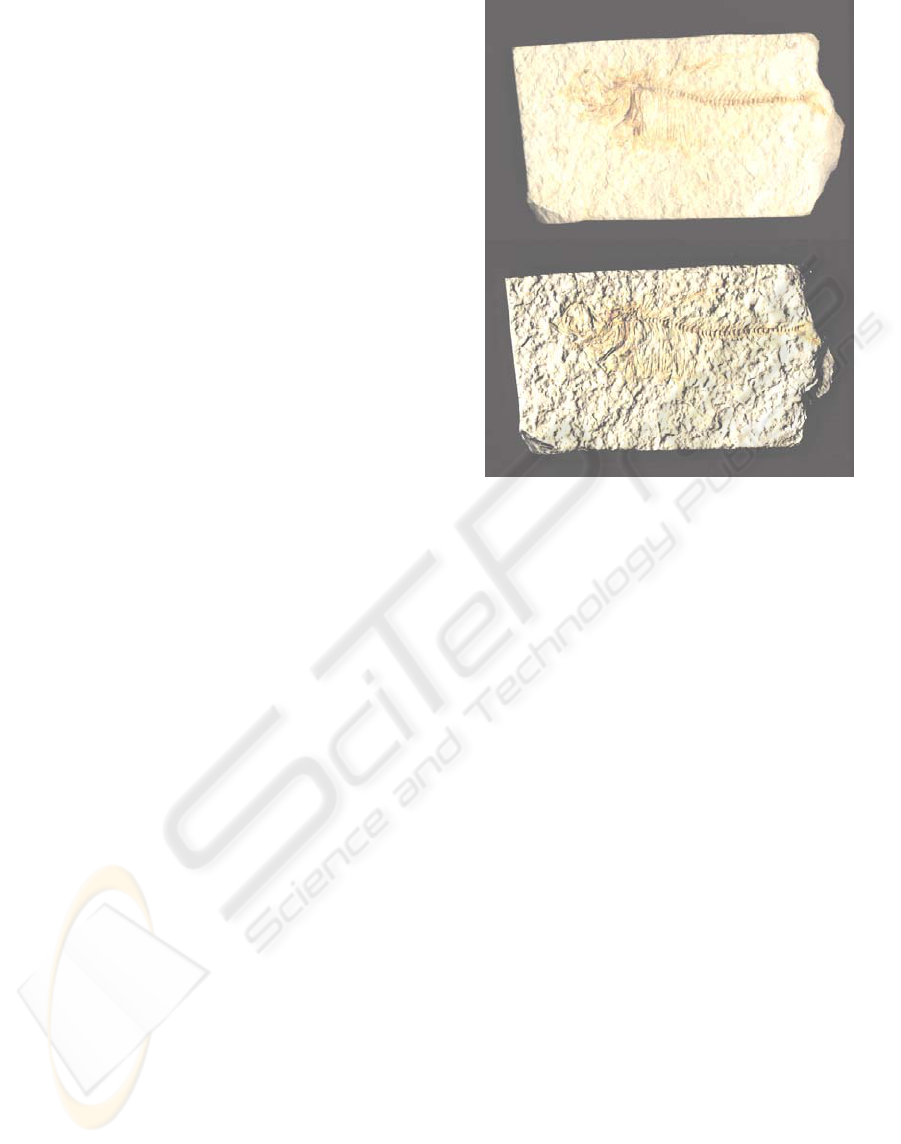
Figure 14: Top: The first of the four scans shown in Fig. 3.
Bottom: Interactively relit to enhance surface detail.
ACKNOWLEDGEMENTS
Justin Tehrani with Hewlett-Packard’s Imaging and
Printing Group in Ft. Collins, Colorado was
instrumental in initiating the investigation into the
feasibility of recovering shape information from
multiple lighting. Greg Taylor, also with Hewlett-
Packard’s Imaging and Printing Group, modified a
Scanjet 4890 to allow us to control the bulbs
independently. Dan Gelb at Hewlett-Packard
Laboratories, Palo Alto collaborated on developing
the relighting methods that led to this work.
REFERENCES
Barsky, S., and Petrou, M. 2003. The 4-Source
Photometric Stereo Technique for Three-Dimensional
Surfaces in the Presence of Highlights and Shadows,
IEEE Transaction on Pattern Analysis and Machine
Intelligence, Vol. 25, No. 10, pp. 1239-1252.
Bergman, R., Maurer, R., Nachlieli, H., Ruckenstein, G.,
Chase, P., and Greig, D. 2007. Comprehensive
Solutions for Automatic Removal of Dust and
Scratches from Images, Journal of Electronic Imaging.
Brown, B., Toler-Franklin, C., Nehad, D., Burns, M.,
Dobkin, D., Vlachopoulos, A., Doumas, C.,
Rusinkiewicz, S., Weyrich, T., “A System for High-
Volume Acquisition and Matching of Fresco
Fragments: Reassembling Theran Wall Paintings”,
PHOTO REPAIR AND 3D STRUCTURE
FROM FLATBED SCANNERS
49

ACM Transactions on Graphics, Vol. 27, No. 3,
pp.83:1-9, August 2008.
Buades, A., Coll, B., and Morel, J. 2005. A Review of
Image Denoising Algorithms, With a New One,
Multiscale Modeling and Simulation (SIAM
interdisciplinary journal), Vol 4 (2), pp. 490 - 530.
Chantler, M., and Spense, A. 2004. Apparatus and Method
for Obtaining Surface Texture Information, Patent GB
0424417.4.
DIGITAL ICE™, Eastman Kodak Company,
http://asf.com/products/ice/FilmICEOverview/.
Efros, A., and Leung, T. 1999. Texture Synthesis by Non-
parametric Sampling. In Proceedings of IEEE
Internation Conference on Computer Vision,
September.
Fattal, R., Agrawala, M., and Rusinkiewicz, S. 2007.
Multiscale Shape and Detail Enhancement from
Multiple-light Image Collections, ACM Transactions
on Graphics, 26 (3).
Freeth, T., Bitsakis, Y., Moussas, X., Seiradakis, J.,
Tselikas, A., Mangou, H., Zafeiropoulou, M.,
Hadland, R., Bate, D., Ramsey, A., Allen, M.,
Crawley, A., Hockley, P., Malzbender, T., Gelb, D.,
Ambrisco, W., and Edmunds, M. 2006. Decoding the
Ancient Greek Astronomical Calculator known as the
Antikythera Mechanism, Nature, Vol. 444, Nov. 30,
pp. 587 – 591.
Gardner, A., Tchou, C., Hawkins, T., and Debevec, P.
2003 Linear Light Source Reflectometry, ACM
Transactions on Graphics, Vol. 22, No. 3, pp. 749-758.
Hammer, O., Bengston, S., Malzbender, T., and Gelb, D.
2002. Imaging Fossils Using Reflectance
Transformation and Interactive Manipulation of
Virtual Light Sources, Palaeontologia Electronica ·
August 23.
Hastie, T., Tibshirani, R., and Friedman, J. 2001. The
Elements of Statistical Learning - Data Mining,
Inference, and Prediction. Springer-Velag.
Hewlett-Packard G4050 Photo Scanner, 2007.
www.hp.com.
Horn, P. 1986. Robot Vision, MIT Press, ISBN 0-262-
08159-8.
Klette, R., Schluns, K., and Koschan, A. 1998. Computer
Vision: Three-Dimensional Data from Images,
Springer –Verlag.
Kschischang, F. R., Frey, B. J., and Loeliger, H. A. 2001.
Factor Graphs and the Sum-Product Algorithm, IEEE
Transaction on Information Theory, Vol. 47, No. 2.
Malzbender, T., Gelb, D., and Wolters, H. 2001.
Polynomial Texture Maps. In Proceedings of ACM
Siggraph 2001, ACM Press / ACM SIGGRAPH, New
York. E. Fiume, Ed., Computer Graphics Proceedings,
Annual Conference Series, ACM, 519-528.
Medioni, G., Lee,M., and Tang, C. 2000. A Computational
Framework for Segmentation and Grouping, Elsevier.
Onn, R., and Bruckstein, A. 1990 Integrability
Disambiguates Surface Recovery in Two-Image
Photometric Stereo, International Journal of Computer
Vision, vol. 5, pp. 105-113.
Petrovic, N., Cohen, I., Frey, B. J., Koetter, R., and
Huang, T. S. 2001. Enforcing Integrability for Surface
Reconstruction Algorithms Using Belief Propagation
in Graphical Models, 2001 IEEE Conf. on Computer
Vision and Pattern Recognition, vol. 1, pp. 743-748.
Schubert, R. 2000. Using a Flatbed Scanner as a
Stereoscopic Near-Field Camera, IEEE Computer
Graphics and Applications, pp. 38-45.
Toler-Franklin, C., Finkelstein, A., and Rusinkiewics, S.
2007. Illustration of Complex Real-World Objects
using Images with Normals, International Symposium
on Non-Photorealistic Animation and Rendering.
Tu, P., and Mendonca, P. R. S., 2003. Surface
Reconstruction via Helmholtz Reciprocity with a
Single Image Pair, Proc. of 2003 IEEE Computer
Society Conference on computer Vision and Pattern
Recognition (CVPR’03), pp. 541-547.
Yang, J., Ohnishi, N., and Sugie, N. 2003. Two Image
Photometric Stero Method, Proc. SPIE, Intelligent
Robots and Computer Vision XI, Vol. 1826, pp. 452-
463.
VISAPP 2009 - International Conference on Computer Vision Theory and Applications
50
