
INTERACTIVE JELLYFISH ANIMATION USING SIMULATION
Dave Rudolf
Department of Computer Science, University of Saskatchewan, Saskatoon, Canada
PhaseSpace Inc., San Leandro, USA
David Mould
Department of Computer Science, University of Saskatchewan, Saskatoon, Canada
School of Computer Science, Carleton University, Ottawa, Canada
Keywords:
Jellyfish, Marine invertebrates, Physics-based animation, Fluid dynamics.
Abstract:
This paper presents an automatic animation system for jellyfish that accounts for interaction between the
organism and its surroundings. We endeavor to model the jellyfish’s morphology, as well as its achieved
thrust. We physically simulate the elastic body of the jellyfish and its surrounding sea water. We use a modified
immersed boundary method to combine spring-mass systems and a grid-based semi-Lagrangian fluid solver.
The resulting simulations are efficient with an acceptable compromise in physical accuracy. We reduce our
model for axially symmetric species to 2D, and extrapolate the results to 3D. We add detail to the 3D shape
with noise that is inspired by empirical observations of real jellyfish. We also suggest suitable contraction
functions so that our virtual jellyfish propells itself within the water in a manner similar to the real organism.
The resulting system is capable of animating jellyfish in real-time on modest desktop hardware.
1 INTRODUCTION
Seascapes are becoming more common in the com-
puter animation industry following the popularity of
productions such as Pixar’s Finding Nemo (2003). As
well, advances in numerical techniques and hardware
are making physical simulation of virtual environ-
ments more feasible. Simulation has the advantage of
automatically animating interactions between charac-
ters and their environments. This paper proposes an
animation system for jellyfish that uses computational
fluid dynamics so that the virtual organism can affect
its environment, and vice versa.
We are interested in the unique mode of jet-
propelled locomotion exhibited by jellyfish, as illus-
trated in Figure 1. This style of motion is largely not
understood either by computer scientists or by marine
biologists. Beer et al. (1997) suggest that the study of
relatively simple animals such as jellyfish will yield a
better idea of how to animate more complicated de-
formable marine life.
Physiologically, jellyfish are not overly complex:
they are invertebrates with a simple nervous sys-
tem (Arai, 1997). However, their mode of locomotion
is still difficult to model numerically, owing to the
Figure 1: Captured footage of a real jellyfish swimming.
combination of the organism’s elastic body and the
surrounding incompressible fluids (Stockie & Wetton,
1999). We use simulation not for accuracy reasons,
but so that our virtual jellyfish can physically interact
with the water around it. Our simulations use a mass-
spring system (Terzopoulos, Platt, Barr & Fleischer,
1987) to represent the elastic body of the jellyfish, and
a semi-Lagrangian fluid solver (Stam, 1999) for the
surrounding sea water. The two representations are
coupled using the immersed boundary method (Pe-
skin, 2002). This method is effective for our system.
However, a full 3D simulation would still be quite ex-
pensive. Thus, we make reductions to our model.
Many species of jellyfish are axially symmetric,
which we exploit by simulating only a low-resolution
2D slice. By doing so, we are able to animate jelly-
fish in an appealing, convincing, and efficient manner.
We then extrapolate the 2D results to a higher resolu-
tion 3D model. Since a na
¨
ıve 3D extrapolation would
lack the geometric complexity seen in real jellyfish,
241
Rudolf D. and Mould D.
INTERACTIVE JELLYFISH ANIMATION USING SIMULATION.
DOI: 10.5220/0001792402410248
In Proceedings of the Fourth International Conference on Computer Graphics Theory and Applications (VISIGRAPP 2009), page
ISBN: 978-989-8111-67-8
Copyright
c
2009 by SCITEPRESS – Science and Technology Publications, Lda. All rights reserved

we also propose means to add variation back into the
3D geometry, based on observations from the biology
community.
Controlling motor functions is a further challenge.
Jellyfish have a simple muscular structure, but use it
in complex ways that are not well studied. We give
one possible approach to motor control for jellyfish,
based on empirical observation. We focus on the res-
onant gait of jellyfish, which is marked by a regular
swimming action at a rate close to a resonant fre-
quency of the organism and its environment (Megill,
2002). We restrict our interest to fully grown adult
jellyfish, as the organism most actively swims in this
phase of its development.
The main contribution of this paper is our auto-
mated system for animating jellyfish, running on con-
ventional desktop hardware at interactive rates, yet
still accounting for physical interactions between the
jellyfish and its surrounding fluid. Our model incor-
porates the biological aspects of the organism that in-
fluence its locomotion. We also show that a simula-
tion model of jellyfish can effectively be reduced to a
coarse 2D model, while providing methods to extrap-
olate back to a detailed and compelling 3D rendering
model. We modify Peskin’s immersed boundary to be
more suitable for coarse models. Lastly, we also pro-
vide a simple procedural mechanism for controlling
the organism’s physiology in order to achieve loco-
motion.
Our work is most interesting to graphics re-
searchers and tool designers. The animations pro-
duced by our model are convincing to a general au-
dience. Although our particular model would not be
accurate enough for experimental biologists, the biol-
ogy community can draw inspiration from our work
in developing their own simulations of jellyfish.
2 PREVIOUS WORK
Physics-based animation techniques have been devel-
oped for a wide variety of characters: snakes, worms,
and caterpillars (Miller, 1988); fish (Tu & Terzopou-
los, 1994); and, of course, human beings (Hodgins,
Wooten, Brogan & O’Brien, 1995). Jellyfish have
previously been animated through procedural tech-
niques and key-framing (Pixar Animation Studios,
2003). These techniques do not easily model two-
way interactions between the jellyfish and their envi-
ronment.
Particle-based approaches such as mass-spring
systems (Terzopoulos, Platt, Barr & Fleischer, 1987;
Tu & Terzopoulos, 1994) can be used to simulate elas-
tic bodies. Thus, particle-based fluid representations,
such as smoothed particle hydrodynamics (Desbrun &
Gascuel, 1996), might seem tempting. However, SPH
is not as efficient as grid-based methods (Griebel,
Dornseifer & Neunhoeffer, 1998) when simulating
contiguous regions of incompressible fluid, especially
when large forces are acting on the fluid. Stam (1999)
gives an inexpensive grid-based approach that is un-
conditionally stable, though with some numerical
damping.
To couple particle-based solids with grid-based
fluids, the graphics community typically enforces
boundary conditions on the fluid that correspond to
the solid surface’s velocity at each fluid cell. The
most recent work in this vein is that of Robinson-
Mosher et al. (2008), which increases the stability
of simulation by strictly enforcing conservation of
momentum. From the mathematics community, Pe-
skin (2002) uses the immersed boundary method to
couple grid-based fluid representations with particle-
based solids. This method is especially interesting to
us because it has been used to model active elastic
bodies, such as the human heart (McQueen & Peskin,
2000), that exert great force on the fluids around them.
Unlike the work of Robinson-Mosher et al. (2008),
the immersed boundary method does not explicitly
prevent fluid from leaking across thin elastic bound-
aries, and performs poorly when the fluid’s free sur-
face intersects the elastic body. However, our jellyfish
are completely submerged, and leakage is quite mini-
mal (Stockie & Wetton, 1999).
As with all physics-based animation techniques,
we need a way to automatically control the bodies that
are in motion. For some creatures (Wu & Popovi
´
c,
2003; Miller, 1988; Tu & Terzopoulos, 1994), simpli-
fied physical systems are used so that the animation
has some semblance of realism, but the animation can
be controlled with a relatively small number of pa-
rameters. Our system is more complex, in that it has
more parameters. A more adaptive controller, such
as a PID controller (Dean & Wellman, 1991), is also
possible; however, tuning the weights of the control
function is not a trivial task.
From the biology community, Megill (2002)
discusses different gaits of jellyfish. Dabiri and
Gharib (2003) provide empirical data on the large-
scale morphology and kinematics of swimming jel-
lyfish. Gladfelter (1972), and Megill (2002) describe
the elastic properties of the organism, and its distri-
bution of muscle fibres. Gladfelter also gives detailed
data on the deformation of jellyfish as they contract.
The symmetry of jellyfish was previously ex-
ploited by Dabiri and Gharib (2003), though they treat
the organism as perfectly symmetric. To generate a
3D model from a 2D slice, we take inspiration from
GRAPP 2009 - International Conference on Computer Graphics Theory and Applications
242

Rasmussen et al. (2003), who animated 3D explosions
by augmenting the flow of 2D simulations with a 3D
periodic noise field. Perlin (Perlin, 2002) gives a sim-
ple means of computing a continuous noise field.
3 A NUMERICAL MODEL OF
JELLYFISH
This section describes our numerical model of jelly-
fish: our mass-spring configuration for of the organ-
ism’s body, and how we incorporate it into a semi-
Lagrangian fluid solver with a modified immersed
boundary method. This section also discusses the bi-
ological aspects of the organism that are involved in
its locomotion, and lastly how we extrapolate and em-
bellish our 3D model.
3.1 Jellyfish Physiology
Figure 2 highlights the anatomy of the organism that
are of interest to this work. A jellyfish swims by
repeatedly contracting its umbrella, producing thrust
by expelling fluid from the subumbrellar cavity. The
tentacles along the aperture of the umbrella add hy-
drodynamic drag. These tentacles are mostly passive
during normal swimming, but are used when hunt-
ing or moving along the ocean floor (Megill, 2002).
Many species of jellyfish are approximately axially
symmetric, where the axis of symmetry runs from the
apex of the umbrella through the center of its aperture.
Shih (1977) lists a large number of different species of
jellyfish, whose umbrellas and tentacles vary in size
and physical configuration.
Figure 2 also depicts the different tissues within
the umbrella itself. The circumferential muscle that
lines the subumbrellar wall is chiefly involved in lo-
comotion. When this muscle contracts, it pulls the
umbrella inward, creating a fluid jet at the aperture of
the umbrella that propels the organism forward.
Joint Mesoglea Bell Mesoglea
Circumferencial Muscle
Subumbrellar
Cavity
Aperture
Mouth
Apex
Tentacle
Figure 2: Vertical and horizontal cross-sections of a medu-
san umbrella.
Figure 3: The non-linear deformation of the umbrella under
the contraction of the circumferential muscle, shown as a
horizontal cross-section.
Aside from the circumferential muscle, the re-
mainder of the umbrella is categorized into two re-
gions: the bell mesoglea and the joint mesoglea, both
essentially passive. The joint mesoglea’s elastic mod-
ulus is roughly 10% the bell mesoglea’s, so that the
when the umbrella is compressed, the joint mesoglea
deforms into ridges, as illustrated in Figure 3. Be-
cause of the ridges, the elastic properties of the um-
brella are not a linear function of the displacement.
Megill (2002) gives us the shape of the stress-strain
profile.
3.2 2D Simulation Model
We want our simulations to capture three aspects of
the jellyfish’s anatomy: the mesoglea; the circumfer-
ential muscle; and the tentacles. We represent the
subumbrellar surface of the organism with a chain
of Hookean springs, and further enforce the struc-
ture of the umbrella with angular springs. Instead
of angular springs, one might be tempted to enforce
relative orientations with small networks of Hookean
springs, similar to the work of Miller (1988), and Tu
and Terzopoulos (1994). However, we experimentally
found that the large number of short springs (relative
to the resolution of our fluid grid) made the system
less stable. Figure 4 shows our mass-spring config-
uration. The circumferential muscle is represented
by linear springs going longitudinally across the um-
brella. These springs exert an inward thrust on the
subumbrellar surface, as the circumferential muscle
does in real jellyfish. To mimic a contraction of this
muscle, we reduce the rest lengths of these springs to
exert force on the subumbrellar wall.
Figure 4 also shows tentacles, represented by two
strands of points on either side of the umbrella, con-
nected with both linear and angular springs. The
size and makeup of jellyfish tentacles can vary widely
among different species and we artistically chose the
physical parameters of the tentacles. We give the ten-
tacles the same elastic modulus as the umbrella, but
with 1/100th the cross-sectional area.
We model the flow of the sea water surrounding
the jellyfish using the incompressible Navier-Stokes
INTERACTIVE JELLYFISH ANIMATION USING SIMULATION
243

equations:
∂~u
∂t
= ν∇
2
~u −~u · ∇~u −
∇p
ρ
+
~
F, ∇ ·~u = 0, (1)
where ~u is the fluid’s velocity field, p is the pressure
field, ρ is the fluid density, ν is the fluid’s kinetic vis-
cosity,
~
F is a field of external forces acting on the
fluid, and ∇ and ∇
2
respectively are spatial gradient
and Laplacian operators. Griebel et al. (1998) give a
thorough explanation of Equation 1.
For our 2D simulation, we use the Cartesian for-
mulation of the Navier-Stokes equation. Since we are
modeling axial symmetry, it may be tempting to use
a cylindrical formulation as given by Acheson (Ache-
son, 1990). However, the axis of symmetry can po-
tentially change constantly, and the two halves of the
slice may not mirror each other exactly.
Sea water is essentially incompressible, and a jel-
lyfish can exert large forces on the fluid within its
cavity. Upholding the incompressibility constraint in
Equation 1 is very important to our system. SPH
methods (Desbrun & Gascuel, 1996) approximate in-
compressibility by introducing strong pressure forces
between fluid particles, increasing the numerical stiff-
ness (and thus the computational expense) of the sim-
ulation. Grid-based methods are more appropriate.
We immerse our mass-spring model of the jellyfish in
a square fluid volume that is ten times the jellyfish’s
diameter, and give the fluid cavity free-slip boundary
conditions, as described by Griebel et al. (1998).
We use the immersed boundary method (Peskin,
2002) to couple the particle-based elastic and the grid-
based fluid representations. In Peskin’s method, the
elastic point-masses are advected along the flow field
of the fluid grid, and the elastic forces of the Hookean
springs are applied to the fluid grid using the force
term
~
F in Equation 1. Peskin uses a smoothing ker-
nel to distribute the forces to several, possibly dozens,
of grid cells near the point-mass. Doing so increases
the cost of simulation, and effectively puts an up-
per limit on the frequency at which the force profile
can vary over the fluid grid. Since we use relatively
coarse grids (i.e., 50×50 or 100 ×100), the frequency
limitation of Peskin’s smoothing kernel can make the
fluid appear artificially viscous around the solid point-
masses. We diverge slightly from Peskin’s method,
and instead distribute the elastic force of a point-mass
onto its four closest grid cells with bilinear interpola-
tion to find the contributions to each corner.
Peskin’s method is known to be numerically stiff,
and Stockie and Wetton (1999) show that semi-
implicit integration schemes yield roughly an order
of magnitude in efficiency. However, we find ex-
perimentally that we gain two orders of magnitude
in speed-up over an explicit scheme, simply by us-
ing the semi-Lagrangian method (Stam, 1999). This
method does not gain us larger time-steps, but merely
decreases the cost of each step. Stam’s method is
unconditionally stable when simulating fluids alone,
but large time-steps can still make the mass-spring
network unstable. Similarly, the Courant-Friedrichs-
Lewy stability criterion (Griebel, Dornseifer & Neun-
hoeffer, 1998) does not predict time-steps that keep
the elastic body stable. Lacking a better measure of
stability, we controlled step sizes with the Courant-
Friedrichs-Lewy condition, using a safety factor of
0.001.
3.3 Muscle Activation
Megill (2002) describes several different gaits of the
jellyfish. We aim to animate the resonant gait, which
involves an organism oscillating at or near the reso-
nant frequency of the system. It is the most common
and most studied gait.
To contract the umbrella, we modify the rest
lengths of the subumbrellar springs. Biology liter-
ature provides no evidence that the organism uses
closed-loop controllers such as those described by
Dean (1991) to induce muscle contractions, but rather
suggests a predictable, cyclical pattern (Megill, 2002;
Dabiri & Gharib, 2003). We thus use Hermite splines
to generate each spring’s rest length over time.
When a jellyfish contracts, it propels itself for-
ward. However, when it expands, it also pulls it-
self backward. For a jellyfish to achieve a net posi-
tive movement over a contraction cycle, the organism
must incur less overall drag in the cycle’s expansion
phase than in the contraction phase. We are unaware
of any literature that details how this drag reduction is
achieved. We suspect that jellyfish make themselves
Figure 4: Our mass-spring network for a jellyfish slice, and
the corresponding contraction functions that we use. Lines
represent Hookean springs. Also, angular springs are used
between points on the tentacles, and around the umbrella,
though not across the umbrella. Each spring’s greyscale
level in the left image corresponds to the contraction func-
tion in the right image with the same grey level.
GRAPP 2009 - International Conference on Computer Graphics Theory and Applications
244

more flat to achieve higher drag, and more rounded to
reduce their drag. In Figure 1, the first three frames
show the jellyfish expanding, and its umbrella shape
is relatively curved. In the fourth frame, the jellyfish
is contracting, and the umbrella appears less curved
and more conical. In order to achieve this morphol-
ogy, we slow the expansion of subumbrellar springs
close to the aperture. We give the Hermite splines for
the contraction functions different slopes in the ex-
pansion phase. Springs closer to the umbrella’s apex
have steeper slopes than those closer to its aperture.
Figure 4 shows our mass-spring model of the jelly-
fish, with the corresponding contraction functions for
each spring.
The frequency of the jellyfish’s contractions has
a direct effect on the organism’s achieved thrust, as
well as its morphology. The resonant frequency of
the system depends mostly on the umbrella’s diam-
eter (Megill, 2002). We experimented with different
contraction frequencies to determine which ones were
optimal for our model. Figure 5 shows the transla-
tional motion of a simulated jellyfish with an umbrella
diameter of 40 mm, but with different contraction fre-
quencies. We get a large maxima in total vertical dis-
placement for a frequency of 0.7 Hz, which agrees
with data measured by Dabiri and Gharib (2003).
3.4 3D Rendering Model
The points in our simulation model represent the sub-
umbrellar surface. To account for the thickness of the
umbrella, we generate the exumbrellar side by pro-
jecting each surface point backward along its normal.
Figure 3 gives suitable thickness values. We then re-
sample the coarse set of points to arbitrary resolutions
by interpolating a cubic spline through the original
point-masses and then the newly generated exumbrel-
lar points.
The subumbrellar points may not be symmetric
Distance Travelled for Several Contraction Frequencies
0.0
0.1
0.2
0.3
0.4
0.5
0.6
0.7
0.8
2018
16
14
12
108
642
0
Time (s)
Distance (m)
f=0.4
f=0.7
f=1.0
f=1.5
f=2.0
Figure 5: Trajectories of several simulated organisms with
different frequencies of contraction.
Figure 6: The results of our 2D simulation; trace particles
show the flow of the fluid around the contracting jellyfish.
within the 2D plane (i.e., the two sides of the um-
brella may not mirror each other). Thus, we cannot
extrapolate the geometry by merely rotating the re-
sults of the slice about the axis of symmetry, as Dibiri
and Gharib (2003) did. Instead, we consider each pair
of points ~x
i
and ~x
j
opposite to each other on the um-
brella. Note that the pairs of points in question re-
sulted from the resampling of the coarse geometry.
We define an axis of rotation for each pair, which goes
through the center of the line segment between the
points ~x
i
and ~x
j
, and is orthogonal to that line seg-
ment. We use the same disc extrapolation scheme for
generating tentacles along the 3D aperture of the um-
brella. Figure 7 illustrates our process of extrapolat-
ing circular area from pairs of points in our 2D model.
Our disc-based extrapolation generates an artifi-
cially smooth volume. Although a given species may
be roughly symmetric, individual jellyfish are not ex-
actly so, as seen in Figure 8. To add variation to our
rendering model, we perturb each point~x
i, j
on the um-
brella’s surface by some scalar distance c
i, j
in the di-
rection of its surface normal ~n
i, j
, where (i, j) is the
azimuth and elevation indices of the point.
Several factors can cause small-scale asymme-
tries. Periodic features in the underlying umbrella ge-
ometry are particular to the species of jellyfish (Shih,
Figure 7: An example of point pairs along the 2D umbrella
slice that have been extrapolated to 3D discs. For each point
pair, the line between them is bisected orthoganally by the
rotational axis, and a disc results from rotating those points
about that axis.
INTERACTIVE JELLYFISH ANIMATION USING SIMULATION
245
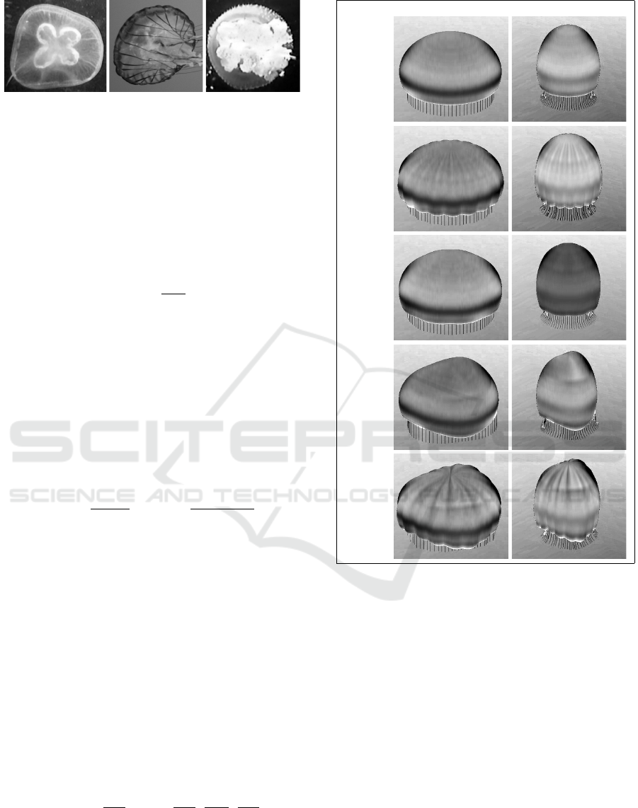
Figure 8: Jellyfish that are not exactly symmetric.
1977), as seen in the right-most two images in Fig-
ure 8. For these structural patterns, we define func-
tions to generate the desired appearance:
c
str
i, j
= α
str
sin( f σ
j
), or c
str
i, j
= α
str
|sin( f σ
j
)|, (2)
where α
str
is an artistically-chosen scale factor, f is
the frequency of the variation, and σ
j
is the longitu-
dinal angle of points~x
i, j
for all values of i. This angle
can be expressed as:
σ
j
= 2π
j
j
max
. (3)
Another type of variation, seen in Figure 3, is caused
by the nonuniform elastic properties of the jellyfish’s
mesoglea, which produce ripples across the contract-
ing umbrella. This variation is also roughly sinu-
soidal, though its amplitude depends on the amount of
umbrellar contraction. To account for contraction ef-
fects, we use a spring’s uncontracted rest length l
r
and
its current length l
c
to define a contraction coefficient
that is at 1 when l
c
= l
r
, and 0 when l
c
= (0.46)l
r
.
Then, the overall displacement of the umbrella hull
can be described:
c
cmp
i, j
= α
cmp
l
c
− γl
r
l
r
− γl
r
n
η + κ
sin(σ
j
) + 1
2
o
. (4)
The constants η = (1.34 −1), γ = (1 −0.54), and κ =
(1.51 − 1.34) all come from Figure 3. Note that only
points on the exumbrellar surface are affected in this
manner.
Lastly, asymmetric differences arise between in-
dividuals of the same species. We mimic this varia-
tion artistically using Perlin noise (2002). We control
the frequency of each dimension of the noise func-
tion independently, with the intent of qualitatively ap-
proximating the look of a target jellyfish. Since the
mesoglea is thicker at the top of the umbrella, it is
more resistant to deformation in this region. We at-
tenuate the amplitude of the noise function for points
near the peak of the umbrella. Our expression for
the displacement of the umbrella points due to non-
periodic variation is as follows:
c
noise
i, j
= α
noise
i
i
max
∗ Q
P
2i
i
max
,
8 j
j
max
,
t
100
, (5)
where t is the simulation time, and Q
P
is the Perlin
noise field. We apply this displacement to both sub-
umbrellar and exumbrellar points, and also tentacle
points.
Expanded Contracted
3D
Ex-
trap.
Struct.
Compr.
Noise
All
Figure 9: Our 3D extrapolation, and the types of noise that
we apply to the hull of the umbrella. The first column of im-
ages shows the jellyfish at its expanded (rest) configuration,
and the bottom row shows the contracted configuration.
4 RESULTS
Figure 10 shows a full cycle of our jellyfish swim-
ming. We render the final model with a simple Lam-
bertian surface lighting model. We find the motion
of our jellyfish to be quite convincing, comparable
to previous animations of jellyfish such as in Pixar’s
“Finding Nemo” (2003). Our method has the advan-
tage that the resulting animation’s upward movement
is more closely tied to the contraction of the organ-
ism, and the virtual organism interacts with its envi-
ronment directly and automatically. Also, our mor-
phology appears to more closely resemble that of real
GRAPP 2009 - International Conference on Computer Graphics Theory and Applications
246
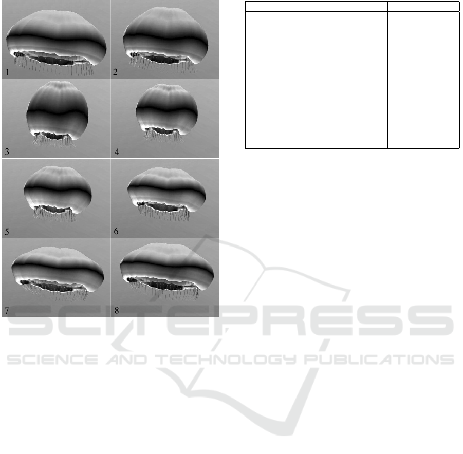
Figure 10: A sequence of frames from our animation sys-
tem.
jellyfish.
Although accuracy is not the primary concern of
our model, we discuss it briefly here. We found
experimentally that our model has a similar reso-
nant frequency to captured data from Dabiri and
Gharib (2003). However, the motion that our model
generates is noticeably different from empirical data
of jellyfish. Figure 5 shows high-frequency motion
that has a higher amplitude than that shown by Dabiri
and Gharib (2003), meaning that our model’s posi-
tion oscillates up and down more, relative to its over-
all translational motion.
We are able to achieve real-time animations at 30
to 40 frames per second on modest hardware (AMD
Turion 1.6 GHz processor), depending on the reso-
lution of our 2D simulation and of our 3D extrapo-
lation. We experimentally find that time-steps of the
order of 0.01 seconds begin to hit the stability lim-
its of the system. Each frame must be broken into
multiple simulation steps, but of course, resampling
and 3D extrapolation only needs to be done once per
frame. Figure 11 shows the parameters of our sim-
ulations, and the values that we used to generate the
animations that are featured in this paper.
Parameter Value
Fluid Grid Height/Width (n) 100
Fluid Viscosity (ν) 1.304 ×10
−3
Fluid Density (ρ) 1
Safety Factor for Integration Step Size 0.001
Jellyfish Contraction Frequency 0.7Hz
Jellyfish Diameter 40mm
Jellyfish Height 28mm
Jellyfish Thickness (ϑ) 4mm
Hookean Elastic Modulus 1186Pa
Angular Elastic Stiffness 1.186 N · m/rad
Tentacle Cross-sectional Area Factor 1/100
Structural Variation Scale (α
str
) 0.375 ·ϑ
Compression Variation Scale (α
cmp
) 0.25 ·ϑ
Structural Variation Scale (α
noise
) 2.25 ·ϑ
Figure 11: Parameters of our animation system.
5 CONCLUSIONS AND FUTURE
WORK
We simulate a model of jellyfish numerically, which
accounts for the elastic forces of the organism as it
contracts its muscles, as well as the reaction of the
sea water that surrounds the organism. Simulation al-
lows us to model the direct interaction of the jellyfish
and its environment. We simulate only a 2D vertical
slice of the jellyfish and exploit the axial symmetry
of the organism. We also concentrate on the resonant
gait of an adult jellyfish, in which it contracts at its
submerged natural resonant frequency.
We represent the jellyfish’s flesh and subumbrellar
muscles as a mass-spring system (Terzopoulos, Platt,
Barr & Fleischer, 1987) that consists of a combina-
tion of linear and angular springs. We shorten the rest
lengths of subumbrellar springs to simulate the con-
traction of muscles within the umbrella based on an
artistically chosen periodic function. We account for
sea water with a semi-Lagrangian fluid solver (Stam,
1999) in conjunction with the immersed boundary
method (Peskin, 2002).
We generate a higher resolution model from our
coarse simulations by threading a cubic spline inter-
polant around the simulated point-masses. We then
extrapolate to a 3D surface by defining discs that go
through either side of the jellyfish’s umbrella, and add
several forms of variation to the resulting 3D surface.
These variations are partly based on observations of
real jellyfish, and partly artistic.
Much work could still be done with respect to jel-
lyfish animation. We would like to remove the as-
sumption of axial symmetry, possibly by simulating
multiple 2D slices. Also, jellyfish are capable of other
locomotion modes besides the common resonant gait,
and simulating these would increase the range of mo-
tion of our virtual jellyfish.
INTERACTIVE JELLYFISH ANIMATION USING SIMULATION
247

We still know little about exactly how jellyfish
contract their muscles to achieve jet propulsion. Van
de Panne and Fiume (1993) designed a means of
experimenting with the control processes for sim-
ple creatures using sensor-actuator networks. We
could perhaps leverage this kind of control explo-
ration within the context of jellyfish.
In our work, we have not discussed how some
species of jellyfish are able to reorient themselves.
Megill (2002) states that there are sparse muscle fibres
in the bell mesoglea that are normal to the umbrella’s
surface. These fibres can change the symmetry of the
umbrella and thus effect a course change for the or-
ganism as it swims, though the exact process is not
well understood. So far, we were not able to repro-
duce this phenomenon within our model.
We could improve our rendering of the jellyfish by
considering translucence and bioluminescence, and
by improving our noise model. Also, our rendering
model currently lacks the venous structure visible in
some species of jellyfish.
REFERENCES
Acheson, D. J. (1990). Elementary Fluid Dynamics. Ox-
ford: Oxford University Press.
Arai, M. N. (1997). A Functional Biology of Scyphozoa.
London: Chapman and Hall.
Beer, R. D., Quinn, R. D., Chiel, H. J., & Ritzmann, R. E.
(1997). Biologically inspired approaches to robotics:
what can we learn from insects? Commun. ACM,
40(3), 30–38.
Dabiri, J. O. & Gharib, M. (2003). Sensitivity analysis of
kinematic approximations in dynamic medusan swim-
ming models. Journal of Experimental Biology, 206,
3675–3680.
Dean, T. & Wellman, M. (1991). Planning and Control.
San Francisco: Morgan Kaufmann Publishers.
Desbrun, M. & Gascuel, M.-P. (1996). Smoothed particles:
a new paradigm for animating highly deformable bod-
ies. In Proceedings of the Eurographics workshop on
Computer animation and simulation ’96, (pp. 61–76).,
New York, NY, USA. Springer-Verlag New York, Inc.
Gladfelter, W. B. (1972). Structure and function of the loco-
motory system of polyorchis montereyensis (cnidaria,
hydrozoa). Helgolaender Wiss. Meeresunters, 23, 38–
79.
Griebel, M., Dornseifer, T., & Neunhoeffer, T. (1998). Nu-
merical Simulation in Fluid Dynamics: a practical in-
troduction. Philadelphia: Society for Industrial and
Applied Mathematics.
Hodgins, J. K., Wooten, W. L., Brogan, D. C., & O’Brien,
J. F. (1995). Animating human athletics. In Proceed-
ings of SIGGRAPH ’95, (pp. 71–78). ACM Press.
McQueen, D. M. & Peskin, C. S. (2000). Heart simula-
tion by an immersed boundary method with formal
second-order accuracy and reduced numerical viscos-
ity. In Mechanics for a New Millennium: Proceed-
ings of the International Conference on Theoretical
and Applied Mechanics (ICTAM), (pp. 429–444).
Megill, W. M. (2002). The biomechanics of jellyfish swim-
ming. Ph.D. Dissertation, Department of Zoology,
University of British Columbia.
Michiel van de Panne, E. F. (1993). Sensor-actuator net-
works. In Proceedings of SIGGRAPH ’93, (pp. 335–
342)., New York, NY, USA. ACM Press.
Miller, G. S. P. (1988). The motion dynamics of snakes
and worms. In Proceedings of SIGGRAPH ’88, (pp.
169–173). ACM Press.
Perlin, K. (2002). Improving noise. In Proceedings of SIG-
GRAPH ’02, (pp. 681–682)., New York, NY, USA.
ACM Press.
Peskin, C. (2002). The immersed boundary method. Acta
Numerica 11, 479–517.
Pixar Animation Studios, W. D. P. (2003). Finding Nemo
motion picture. DVD.
Rasmussen, N., Nguyen, D. Q., Geiger, W., & Fedkiw, R.
(2003). Smoke simulation for large scale phenomena.
ACM Trans. Graph., 22(3), 703–707.
Robinson-Mosher, A., Shinar, T., Gretarsson, J., Su, J., &
Fedkiw, R. (2008). Two-way coupling of fluids to
rigid and deformable solids and shells. In SIGGRAPH
’08: ACM SIGGRAPH 2008 papers, (pp. 1–9)., New
York, NY, USA. ACM.
Shih, C. T. (1977). A Guide to the Jellyfish of Canadian
Atlantic Waters. Number 5. Ottawa, Canada: National
Museum of Natural Sciences.
Stam, J. (1999). Stable fluids. In Proceedings of SIG-
GRAPH ’99, (pp. 121–128)., New York, NY, USA.
ACM Press/Addison-Wesley Publishing Co.
Stockie, J. M. & Wetton, B. R. (1999). Analysis of stiffness
in the immersed boundary method and implications
for time-stepping schemes.
Terzopoulos, D., Platt, J., Barr, A., & Fleischer, K. (1987).
Elastically deformable models. In Proceedings of
SIGGRAPH ’87, (pp. 205–214). ACM Press.
Tu, X. & Terzopoulos, D. (1994). Artificial fishes: Physics,
locomotion, perception, behavior. Computer Graph-
ics, 28(Annual Conference Series), 43–50.
Wu, J. & Popovi
´
c, Z. (2003). Realistic modeling of bird
flight animations. ACM Trans. Graph., 22(3), 888–
895.
GRAPP 2009 - International Conference on Computer Graphics Theory and Applications
248
