
CURL-GRADIENT IMAGE WARPING
Introducing Deformation Potentials for Medical Image Registration using
Helmholtz Decomposition
Michael Sass Hansen, Rasmus Larsen
Department of Informatics and Mathematical Modelling, Technical University of Denmark, Copenhagen, Denmark
Niels Vorgaard Christensen
Institute of Mathematics, University of Copenhagen, Copenhagen, Denmark
Keywords:
Image registration, Morphometry, Helmholtz decomposition.
Abstract:
Image registration is becoming an increasingly important tool in medical image analysis, and the need to
understand deformations within and between subjects often requires analysis of obtained deformation fields.
The current paper presents a novel representation of the deformation field based on the Helmholtz decompo-
sition of vector fields. The two decomposed potential fields form a curl free field and a divergence free field.
The representation has already proven its worth in fluid modelling and electrostatics, and we show it also has
desirable features in image registration and morphometry in particular. The potentials are shown to a offer
decoupling of the two potential fields in both elastic and fluid image registration. For morphometry applica-
tions, we show that when decomposing the deformation field in symmetric and antisymmetric parts, the vector
potential alone describes the vorticity, and the scalar gradient potential gives a first-order approximation to the
determinant of the Jacobian.
We provide some insight into the behavior of curl and divergence representation of the warp field by con-
structed examples and by a demonstration on real medical image data. Our theoretical findings are readily
observable in our empirical experiment, which further illustrates the benefit of the parametrization.
1 INTRODUCTION
Image registration is becoming an increasingly impor-
tant tool in medical image analysis, and the need to
understand deformations within and between subjects
often requires analysis of obtained deformation fields
(Studholme and Cardenas, 2007; Davatzikos et al.,
1996).
The image registration task has been approached
in many different ways. It can be achieved by calcula-
tion of dense deformation fields using nonparametric
methods as described by Modersitzki (Modersitzki,
2004). Vermuri et al. proposed a levelset represen-
tation of the deformations (Vemuri et al., 2003). For
more than a decade parametric representation of the
deformation fields has also been very popular in the
literature, where two prominent examples are the co-
sine kernels presented by Cootes et al. (Cootes et al.,
2004), and the Cubic B-spline kernels used by Rueck-
ert et al. (Rueckert et al., 2003). The later intro-
duces a certain smoothing by the finite size of the
parametric kernel functions, but often further regu-
larization is introduced. Haber and Modersitzki in-
troduced regularization terms to ensure displacement
regularity (Haber and Modersitzki, 2007). Elastic reg-
istration is a popular form of regularization, originat-
ing from continuum mechanics as described by Chris-
tensen and Johnson (Christensen et al., 1997) and by
Kybic et al. (Kybic and Unser, 2003).
In the subsequent morphometry it has been shown
that the Jacobian of the deformation field is very im-
portant under a Gaussian random field assumption
on the deformation field (Joshi, 1997). Chung et al.
have investigated different measures of morphome-
try, and also introduced a strain-curl representation
of the deformation field, which has interesting rela-
tions to other morphometry measures (Chung et al.,
2001). Hsiao et al. have shown that using a parame-
179
Sass Hansen M., Larsen R. and Christensen N. (2009).
CURL-GRADIENT IMAGE WARPING - Introducing Deformation Potentials for Medical Image Registration using Helmholtz Decomposition.
In Proceedings of the Fourth International Conference on Computer Vision Theory and Applications, pages 178-185
DOI: 10.5220/0001793301780185
Copyright
c
SciTePress

terizing of the deformation field by its divergence and
curl makes it less prone to grid folding than B-spline
representation, while it allows for an efficient and sta-
ble optimization (Hsiao et al., 2008). Kohlberger et
al. have used potential functions for motion estima-
tion of fluids (Kohlberger et al., 2003).
In Section 2 we propose a new parametric repre-
sentation of the deformation field, which is based on
the Helmholtz decomposition of vector fields. In the
following we show how this representation can also
be parameterized by smooth kernels, how it can be
considered a natural representation for elastic image
registration, we show how it can be given a strong in-
terpretation in morphometry, and finally we point out
how the numerical stability and smoothness obtained
by Hsiao et al. (Hsiao et al., 2008) can also be reached
by our representation.
We have demonstrated an implementation of the
presented method on MRI Corpus Callosa images
from the midsagittal plane in Section 3.
2 METHODS
We present the developed methodology by introduc-
ing the Helmholtz decomposition representation in
Section 2.1, with some intuitive demonstration of the
introduced potential functions. Subsequently we give
theoretical motivations by formulating simple elastic-
ity regularization in Section 2.2, morphometric inter-
pretation in Section 2.3, and finally we demonstrate
properties for optimization in Section 2.4.
2.1 Helmholtz Decomposition of Vector
Fields - Introducing Two New
Deformation Potentials
We define a warp function ϕ as the mapping between
two 3-dimensional images, the image I and the ref-
erence R, ϕ : R
3
→ R
3
, which satisfies that the point
x in the reference R corresponds to the point ϕ(x)
in the image I. The important aspect of this defini-
tion is that that ϕ can be considered a vector field.
For medical image analysis purposes we can further-
more assume that the vector field is smooth, as this
will usually be our best assumption for the anatomi-
cal topology. These considerations also holds for the
deformation field, u, which we define as the differ-
ence from the identity warp, such that ϕ = x + u.
We apply the Helmholtz decomposition to the de-
formation field, using the fact that a vector field,
which is twice continuously differentiable and with
rapid enough decay at infinity, can be split into a sum
of the gradient of a scalar function and the curl of a
vector function (Griffith, 1999)
u(x) = ∇V(x) + ∇× A(x), (1)
where V : R
3
→ R and A : R
3
→ R
3
are scalar
and vector potentials functions respectively. Sections
2.2,2.3 and 2.4 all deal with specific properties of this
representation by potentials. Because they are new in
the field of medical image analysis, we start by ex-
ploring some of the immediate properties of these po-
tentials. Recall that the deformation field is merely
a sum of the two, then we shall explore the gradient
potential V, and the curl potential A one at a time.
2.1.1 The Gradient Potential V
The gradient potential is roughly speaking govern-
ing local contraction or expansion, this is in partic-
ular true in the presence of sufficiently small defor-
mations. The same potential is used in electrostatics
to describe the electrical potential. In Figure 1 gra-
dient potentials and their impact on the deformation
field are illustrated. It can be observed how a positive
versus a negativegradient results in expansion or con-
traction of the deformation fields. Two-dimensional
functions are used for the purpose of illustration.
2.1.2 The Curl Potential A
The curl potential field is the equivalent to the mag-
netic potential field in electrostatics. It is describing
purely divergence-freedeformations, which can be in-
terpreted as vortices. In Figure 2 different curl po-
tentials and their impact on the deformation field are
illustrated. For the purpose of illustration only the z-
component of the curl potential A is illustrated, and
only the impact on the x,y directions of the deforma-
tion field are illustrated.
2.2 Elastic Registration
As previously mentioned, the elastic potential is often
used for image registration, which is often based on a
physical motivation in terms of an elastic tissue model
(Christensen et al., 1997; Kybic and Unser, 2003).
Regularization is usually formulated by a potential S
and differential operators B (Haber and Modersitzki,
2007)
S [u] =
Z
Ω
hB [u],B [u]i
R
d
dx . (2)
The corresponding Gâteaux derivative is then given
by
d
u;v
S [u] =
Z
Ω
hA [u](x),v(x)i
R
d
dx , (3)
VISAPP 2009 - International Conference on Computer Vision Theory and Applications
180
50
100
150
0
50
100
0
500
1000
x
2
x
1
V−potential
Warped grid
Reference grid
50
100
150
0
50
100
−1000
−500
0
x
1
x
2
V−potential
Warped grid
Reference grid
50
100
150
0
50
100
0
10
20
x
1
x
2
V−potential
50
100
150
0
50
100
−20
−10
0
x
1
x
2
V−potential
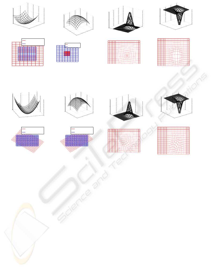
Figure 1: Gradient potentials, V, are illustrated in the upper row, and their impact on the deformation fields are shown below.
The quadratic surfaces with constant curvature produce global scaling, and the potentials with local variations produce a local
contraction or expansion.
50
100
150
0
50
100
0
500
x
1
x
2
A
3
−potential
Warped grid
Reference grid
50
100
150
0
50
100
−1000
−500
0
x
1
x
2
A
3
−potential
Warped grid
Reference grid
50
100
150
0
50
100
0
10
20
x
1
x
2
A
3
−potential
50
100
150
0
50
100
−20
−10
0
x
1
x
2
A
3
−potential
Figure 2: z-component, A
z
of curl potential fields A are shown in the upper row, and the impact on the x, y coordinates
of the deformation field are shown below. A quadratic potential with constant curvature produces a global rotation of the
deformation field, and a local change to the potential results in a local vortex in the deformation field.
where A = B
∗
B . For the elastic potential this Navier-
Lamé operator is given by
A = B
∗
B [u] = µ∆u + (λ + µ)∇(∇· u ) (4)
2.2.1 Elastic Registration of the Helmholtz
Decomposition
We examine how the elastic potential affects the
Helmholtz decomposition of the warp field, and
straightforward calculations give
P [u] =
Z
Ω
µ
3
∑
a,b=1
ε
2
ab
+ (µ+ λ)(∇ · u)
2
dx , (5)
where ε
ij
= δu
i
/δx
j
+δu
j
/δx
i
. Now u = ∇V +∇×A
and
A [u] = µ∆u + (λ + µ)∇(∇ · u)
= µ∆(∇V + ∇ × A)
+(λ+ µ)∇(∇· (∇V + ∇ × A))
= (2µ+ λ)∇∆V + µ∆∇× A. (6)
This is a rather remarkable result, since we can now
decouple the two potentials. Let λ
1
= 2µ+λ and λ
2
=
µ, then
A [u] = λ
1
∇∆V + λ
2
∆∇× A (7)
and replacing the Lamé constants µ and λ by λ
1
and
λ
2
, we have a clear notion of how to interpret the two
regularization parameters. Not all values of λ
1
and λ
2
have meaning in a physical material-property sense
(as goes for a negative µ as well), which should be
considered. It can be argued, though, that the com-
putational model should be extended to include these
cases as well (Modersitzki, 2004). All derivations are
also valid if we had differentiated in the time-domain,
so our potential representation has the same advan-
tages in fluid image registration.
2.3 Deformation-based Morphometry
Following Chung et al. we shall assume that the dis-
placement field u is a smooth function in time, cap-
turing the variation in shape over time (Chung et al.,
CURL-GRADIENT IMAGE WARPING - Introducing Deformation Potentials for Medical Image Registration using
Helmholtz Decomposition
181

2001). In Section 3 we discuss how an artificial time
can be introduced, even when we are doing inter-
subject registration. Introducing deformation fields as
a function of time, u(x,t), the deformation field u at
x + dx can be written using a Taylor expansion
u(x + dx,t) ≈ u(x,t) + J
u
dx , (8)
where J
u
denotes the Jacobian of the deformation
field. It is usually assumed that the Jacobian contains
all information relevant in morphometry, and still fol-
lowing Chung we shall look at a possible decomposi-
tion of it.
2.3.1 Vorticity and Strain of the Jacobian
The Jacobian can be divided into symmetric and anti-
symmetric parts by the following decomposition
∂u
j
∂x
i
=
1
2
∂u
j
∂x
i
−
∂u
i
∂x
j
+
1
2
∂u
j
∂x
i
+
∂u
i
∂x
j
(9)
The first antisymmetric part is termed vorticity and
the second part the strain. Using this (8) may be writ-
ten as
u(x + dx,t) =
u(x,t) −
1
2
∇× u(x,t) × dx + ǫ(x,t)dx , (10)
where the strain matrix is given by ǫ = (ε
ij
) =
1
2
∂u
∂x
+
∂u
∂x
T
. Observe that the vorticity depends
on the A potential alone. Since ∇ × ∇V(x,t) = 0 we
get ∇ × u(x,t) = ∇× ∇ × A(x,t). The diagonal el-
ements of the strain matrix ǫ are in particular given
by
ε
11
=
1
2
∂u
1
∂x
1
+
∂u
1
∂x
1
=
∂
∂A
2
∂x
3
−
∂A
3
∂x
2
+
∂V
∂x
1
∂x
1
(11)
Taking the temporal derivative, the deformation ve-
locity can be written as
∂u(x + dx,t)
∂t
=
∂u(x,t)
∂t
−
1
2
∂
∂t
∇× u(x,t) × dx +
∂ǫ(x,t)dx
∂t
(12)
and in (Chung et al., 2001) it is shown that the first or-
der approximation to the Jacobian determinant is the
sum of the diagonal elements of the strain matrix ǫ;
∂|J
u
|
∂t
≈
∂ε
11
∂t
+
∂ε
22
∂t
+
∂ε
33
∂t
=
∂
∂t
∂
2
V
∂x
2
1
+
∂
2
V
∂x
2
2
+
∂
2
V
∂x
2
3
. (13)
This is seen to depend on the gradient potential alone,
which can be understood, when we consider that this
approximation of the Jacobian determinant is the di-
vergence of the deformation field, ∇· u. In summary
we notice that our introduced representation gives
several simplifications in relating our parameters to
the morphological changes.
2.4 On Stability and Optimization
Hsiao et al. were using the curl and the divergence of
the deformation field as parameters for image regis-
tration. Their experimental results showed this gave
better stability in terms of avoiding grid folding than
using a uniform B-spline parameterization (Hsiao
et al., 2008). In the current setting these quantities are
given by ∇×u = ∇×∇×A and ∇·u = ∇·∇V = ∆V
respectively. The div-curl solver presented could be
applied for our parameterizations as well, disregard-
ing that we are presenting a different regularization
term. However, for the morphometry test in Sec-
tion 3 we have applied a parameterized variational ap-
proach described in Appendix 4, which demonstrates
our method with elastic regularization. We believe
that the method presented in the current work has a
number of advantages. They have to make use of in-
versions of discretized operators to reconstruct the ac-
tual deformation field in the optimization step, which
gives them a registration less prone to folding. We
can simply use the exact differential operators on our
potentials in order to arrive at actual deformations in
our formulation, and use the regularization to enforce
smoothness and invertibility.
3 RESULTS
To demonstrate that the described parameterization
can also be practically implemented, we have imple-
mented a cubic B-spline parameterization of the two
potential fields. The implementation is described in
more detail in Appendix 4, and in the next section we
show results, and hope to add more intuition for the
presented approach through visualization of the po-
tentials on 2D spaces.
3.1 Morphometry on Corpus Callosum
The corpus callosum has been the subject of much
analysis in the field of medical imaging (Davatzikos
et al., 1996; Rueckert et al., 2003). This is probably
because of its relatively simple shape, and the good
contrast in MRI. We have also chosen corpus callo-
sum MR images sampled in the midsagittal plane to
VISAPP 2009 - International Conference on Computer Vision Theory and Applications
182
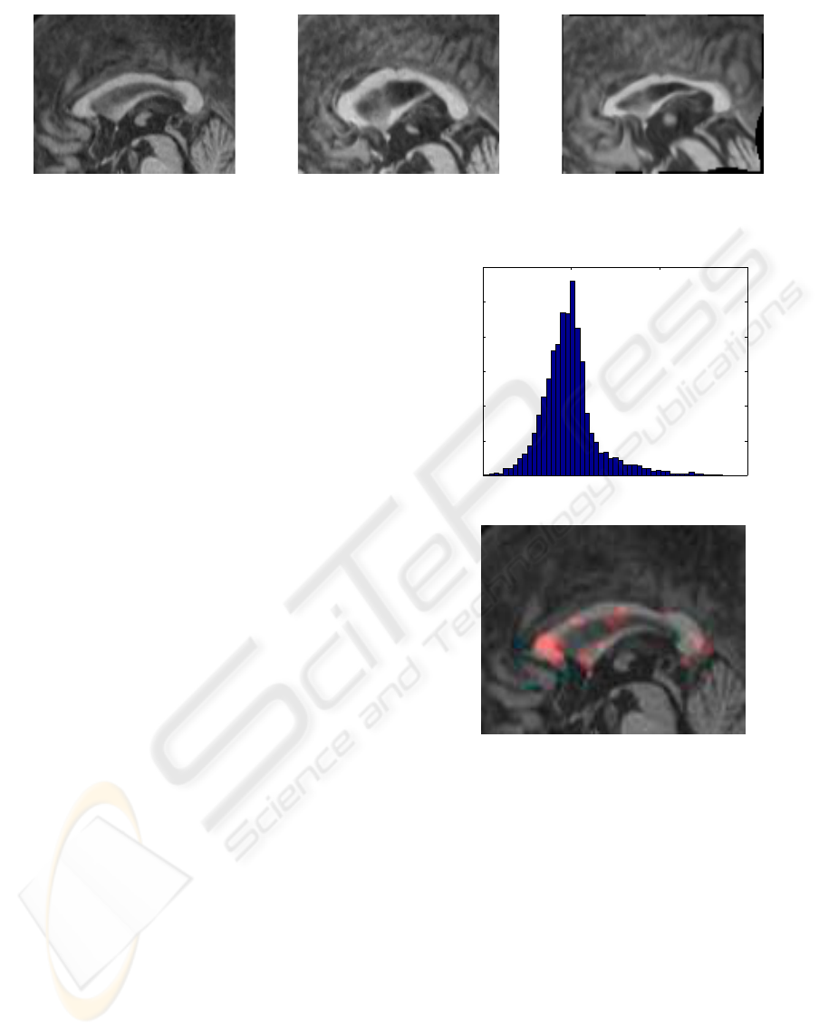
Figure 3: Registration by the proposed parameterization. The image in the middle is registered to the reference (left) and the
result is shown to the right.
demonstrate the presented method. The data set used
for the tests is a subset consisting of 62 MR images
from the LADIS (Leukoaraiosis and DISability) study
(Pantoni et al., 2005) - a pan-European study involv-
ing 12 hospitals and more than 700 patients. In the
optimization we use an artificial time t, when register-
ing one image to another (Modersitzki, 2004). Since
the quantitative analysis is not the major objective of
the current presentation, we put emphasis on illustrat-
ing properties of our potentials. In Figure 3 the image
registration result of one corpus callosum to another
is shown. We analyze the determinant of the defor-
mation field to identify which areas are mostly de-
formed by the registration process. In Figure 4 the
distribution of the determinant and the areas with sig-
nificantly different values are illustrated. It is seen
that the expansion (in this case) is most outspoken in
3 regions of the corpus callosum, which is not so sur-
prising when we investigate the reference, and target
image in Figure 3.
The potentials parameterizing the image registra-
tion are shown in Figure 5. It can be seen that the
V-field is describing expansion and contractions, and
several of the areas with interesting Jacobian deter-
minant in Figure 4 are also seen to represent a rather
strong contraction from the V-potentials. The A-field
is describing rotation - or vortices in the deformation
field.
4 DISCUSSION AND
CONCLUSIONS
In this paper we introduce the theory of a new param-
eterization of 3D deformation fields to the field med-
ical image analysis, using potentials and Helmholtz
decomposition. Similar methods have already proven
valuable in electrostatics and fluid flow estimation
(Griffith, 1999; Kohlberger et al., 2003). We show
the representation can be considered a natural param-
eterization for both elastic and fluid image registration
due to the decoupling of the parameters. For mor-
0 1 2 3
0
200
400
600
800
1000
1200
Figure 4: Above: The distribution of the determinant of the
Jacobian. Below: Region of interest, where the deformation
measured by the determinant, is outside a range of 2 std.
dev..
phometry we have demonstrated that one of the two
potentials directly gives us the vorticity of the defor-
mation field. The determinant gradient field is shown
to be the first-order small-deformation approximation
to the determinant of the Jacobian matrix - probably
the most accepted morphometry measure used. Con-
temporary methods for optimization can supposedly
be adapted to the parameterization (Hsiao et al., 2008;
Kohlberger et al., 2003) and we have outlined our im-
plementation based on finite differences, in Appendix
4.
The major contribution of the paper is primarily
a theoretical one, but we have for demonstration pur-
poses included 2D examples illustrating the relation
CURL-GRADIENT IMAGE WARPING - Introducing Deformation Potentials for Medical Image Registration using
Helmholtz Decomposition
183
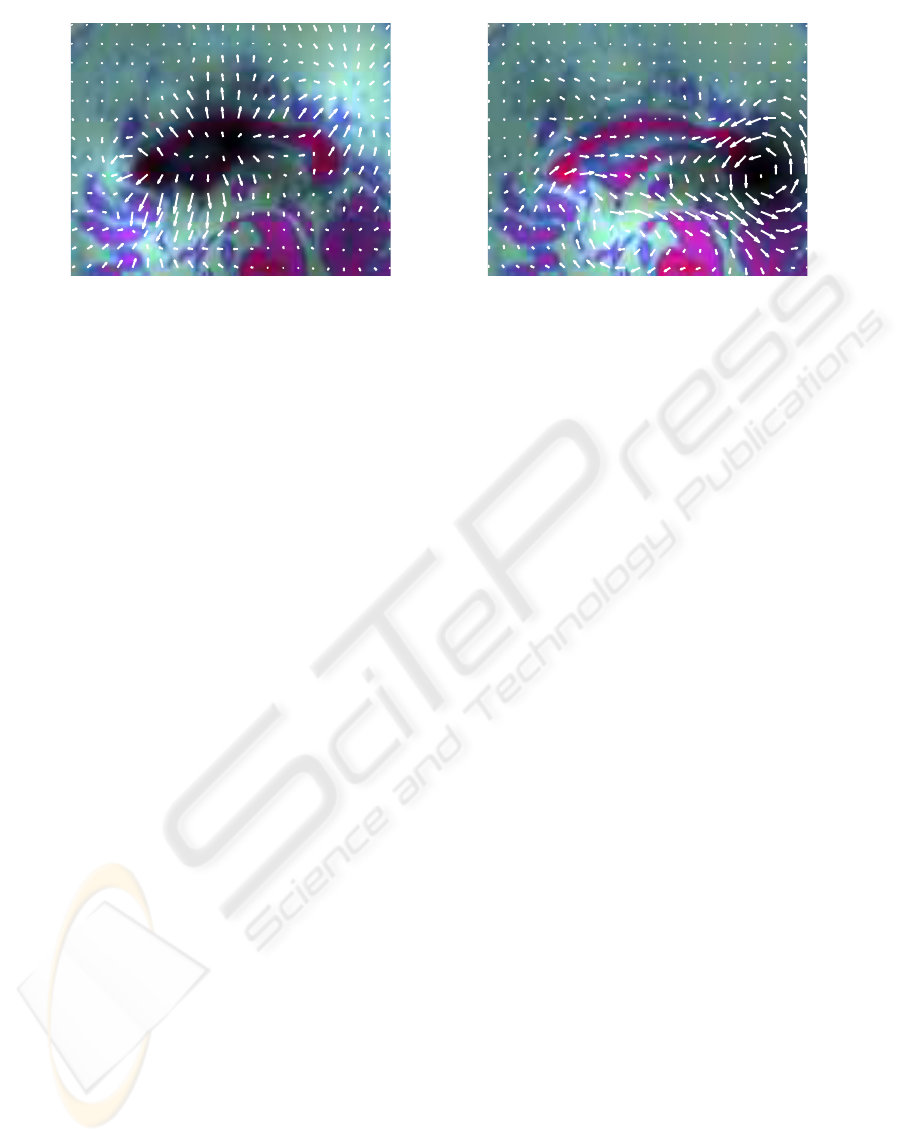
Figure 5: Potential functions shown with images and deformation fields using the HSV colormap. The potential is the value
and the image is the hue. Left: V-potential along with (normalized) deformations this potential causes. Right: A-potential,
and the curl deformations this potential causes.
between the potentials and the observed deformation
fields. It shown that we can get sensible results, where
most of the theoretical observations are readily recog-
nizable from our empirical experiments, and we antic-
ipate many applications in the field of morphometry.
For future work we plan to design quantitative tests
on different medical data sets, to add further empir-
ical validation to the theoretic results demonstrated
in the current paper, and to document the impact on
achieved solutions.
REFERENCES
Christensen, G. E., Joshi, S. C., and Miller, M. I. (1997).
Volumetric transformation of brain anatomy. IEEE
Trans. Med. Imag., 16(6):864–877.
Chung, M. K., Worsley, K. J., Paus, T., Cherif, C., Collins,
D. L., Gieddd, J. N., Rapoport, J. L., and Evans, A. C.
(2001). A unified statistical approach to deformation-
based morphometry. NeuroImage, 14 (3):595–606.
Cootes, T., Twinning, C., and Taylor, C. (2004). Diffeomor-
phic statistical shape models. British Machine Vision
Conference, 1:447–456.
Davatzikos, C., Vaillant, M., Resnick, S., Prince, J.,
Letovsky, S., and Bryan, R. (1996). A computerized
approach for morphological analysis of the corpus cal-
losum. J. Comput Assist Tomogr, 20:88–97.
Griffith, D. (1999). An introduction to electrodynamics.
Prentice Hall.
Haber, E. and Modersitzki, J. (2007). Image registration
with a guaranteed displacement regularity. Interna-
tional Journal on Computer Vision, 71:361–372.
Hsiao, H., Chen, H., Lin, T., Hsieh, C., Chu, M., Liao, G.,
and Zhong, H. (2008). A new parametric nonrigid im-
age registration work based on helmholtz’s theorem.
SPIE Symposium on Medical Imaging 2008.
Joshi, S. (1997). Large deformation diffeomorphisms and
gaussian random fields for statistical characterization
of brain sub-manifolds. PhD thesis, Sever institute of
technology, Washington University.
Kohlberger, T., Étienne Mémin, and Schnörr, C. (2003).
Variational dense motion estimation using the
helmholtz decomposition. 4th International Confer-
ence, Scale Space 2003, 2695:980.
Kybic, J. and Unser, M. (2003). Fast parametric elastic im-
age registration. IEEE Transactions on Image Pro-
cessing, 12(11):1427–1442.
Modersitzki, J. (2004). Numerical methods for image reg-
istration. Oxford Uni. Press.
Pantoni, L., Basile, A. M., Pracucci, G., Asplund, K., Bo-
gousslavsky, J., Chabriat, H., Erkinjuntti, T., Fazekas,
F., Ferro, J. M., Hennerici, M., O’brien, J., Schel-
tens, P., Visser, M. C., Wahlund, L. O., Waldemar, G.,
Wallin, A., and Inzitari, D. (2005). Impact of age-
related cerebral white matter changes on the transition
to disability - the LADIS study: Rationale, design and
methodology. Neuroepidemiology, 24(1-2):51–62.
Rueckert, D., Frangi, A. F., and Schnabel, J. A. (2003).
Automatic construction of 3D statistical deformation
models of the brain using nonrigid registration. IEEE
Transactions on Medical Imaging, 22(8):1014–25.
Studholme, C. and Cardenas, V. (2007). Population based
analysis of directional information in serial deforma-
tion tensor morphometry. Medical Image Computing
and Computer-Assisted Intervention - MICCAI 2007,
4792:311–318.
Vemuri, B. C., Yea, J., Y. Chen, b., and Leonard, C. M.
(2003). Image registration via level-set motion: Ap-
plications to atlas-based segmentation. Medical Image
Analysis, 7(1):1–20.
APPENDIX
In this section we give an overview of implementa-
tion details that are not of great importance to the the-
oretical contributions of this paper. In Section 4 we
introduce the uniform cubic B-spline that are used in
VISAPP 2009 - International Conference on Computer Vision Theory and Applications
184

our implementation. In Section 4 we show some de-
tails on their regularization, and in Section 2.4 we give
some details on how the evaluations can be sped up.
B-spline Representation of Fields
We representedthe potential fields by cubic B-splines,
following (Rueckert et al., 2003). So in summary the
two potential fields are represented as
V =
3
∑
k=0
3
∑
l=0
3
∑
m=0
B
k
(r)B
l
(s)B
m
(t)v
k,l,m
(14)
A =
3
∑
k=0
3
∑
l=0
3
∑
m=0
B
k
(r)B
l
(s)B
m
(t)a
k,l,m
. (15)
Regularization of the B-splines
Applying the elastic constraints (6) to the B-spline
fields, we get for the scalar potential
∇∆V = ∇
3
∑
k,l,m=0
(B
′′
k
(r)B
l
(s)B
m
(t)
+B
k
(r)B
′′
l
(s)B
m
(t) + B
k
(r)B
l
(s)B
′′
m
(t))v
k,l,m
(16)
and for the vector potential we get
∆∇× A =
∆∇×
3
∑
k=0
3
∑
l=0
3
∑
m=0
B
k
(r)B
l
(s)B
m
(t)a
k,l,m
(17)
The regularization of the control points is now deter-
mined by
δS [u]
δv
lkm
= d
u,
δu
δv
klm
S[u] =
Z
Ω
A [u](x),
δu
δv
klm
dx (18)
Optimization
We note that in our parameterized setting, the A -
operator can be written as linear combination of the
parameters A = K
A
p, as can the warp field u = K
u
p.
Using this (18) can be rewritten as
δS [u]
δv
lkm
= d
u,
δu
δv
klm
S[u] =
Z
Ω
(K
A
p)
T
K
u,klm
dx = p
T
Z
Ω
K
T
A
K
u,klm
dx (19)
it is seen that the Gateaux derivative is indeed linear
in the parameters, and the integral needs only be eval-
uated once. The distance measure between reference
and image can for instance be the L
2
-norm
D [R, T;u] =
Z
Ω
[T(x+ u) − R(x)]
2
dx (20)
with the Gateaux derivative
d
u;v
D [R, T;u] =
Z
Ω
hf(x,u(x)),vi
R
d
dx
where f(x, u(x))
=∇T(x+ u(x))(T(x + u(x)) − R(x)) (21)
And the same kernel substitutions can be made as for
the regularization. This facilitates a quick estima-
tion of the deformation field. A further speed up is
gained by implementing a multi-grid cubic B-spline
approach has been used, which also helps avoid lo-
cal minima. In our presented results we used control
point distances of 5, 10 and 20 pixels, respectively.
CURL-GRADIENT IMAGE WARPING - Introducing Deformation Potentials for Medical Image Registration using
Helmholtz Decomposition
185
