
INTERACTIVE IMAGE SEGMENTATION WITH
INTEGRATED USE OF THE MARKERS AND THE
HIERARCHICAL WATERSHED APPROACHES
Bruno Klava and Nina Sumiko Tomita Hirata
Institute of Mathematics and Statistics, University of S
˜
ao Paulo, Rua do Mat
˜
ao, 1010, S
˜
ao Paulo, Brazil
Keywords:
Segmentation, Interactivity, Watershed from markers, Hierarchical watershed.
Abstract:
The watershed transform is a well-known approach for image segmentation. Watershed from markers and
hierarchical watershed are derived from the watershed transform and are suitable for interactive image seg-
mentation: in the former, the user can edit markers and control the segmentation result; in the latter, the user
can select an image partition from a nested set of partitions. We investigate and propose ways to transition
from one approach to other. Such transitions can be used to integrate both approaches in such a way that
allow us to make full use of the strengths of both. We present examples that illustrate the use of the proposed
transitions in conjunction with several interaction possibilities from both approaches.
1 INTRODUCTION
Segmentation is an important stage in almost every
problem involving digital image analysis. The goal
of the segmentation process is to partition the spatial
domain of the image, delimiting the regions of interest
that correspond to the target objects of the analysis in
question.
Since it is not always possible to facilitate the
segmentation process, systems developed to automat-
ically segment images are usually restricted to spe-
cific domains. Even for a particular application pur-
pose, formal specification of the parameters of a seg-
mentation algorithm can be very difficult. In many
cases, in order to obtain a satisfactory result, a post-
processing of the partition (obtained through auto-
matic techniques) is necessary. Moreover, the concept
of a good partition may depend on the purpose of its
use and may be highly subjective.
Interactive segmentation systems are appropriate
to deal with several of these issues. The user can man-
age the segmentation process, having full control over
the level of detail of the desired partition.
The watershed transform (Beucher and Meyer,
1993) is a well-known segmentation tool from math-
ematical morphology. There are two approaches suit-
able for interactive segmentation:
• the watershed from markers approach reduces the
segmentation problem to finding a set of markers
for the regions of interest. The desired partition
can be obtained by interactively handling the set
of markers;
• the hierarchical watershed generates a nested par-
titions set, with partitions of the image at several
resolution levels. The user can navigate through
the hierarchy in order to select a partition with the
desired level of detail for each region of interest.
In the hierarchical watershed approach, the under-
lying structure is the region adjacency graph (RAG)
of an initial fine partition. While pixels correspond
to the atomic units in images, in the hierarchical ap-
proach the atomic units are the regions of the finest
partition. Thus, in any partition derived from the hier-
archy, all resulting regions are unions of some primi-
tive regions.
The formal definition of watershed on graphs
made possible a unifying treatment for segmenta-
tion, regardless of the atomic unit considered (Meyer,
2001b). We say that partitions are at region level pre-
cision if the graph considered is the RAG, whereas
they are at pixel level precision if the graph consid-
ered is the 4 or 8-adjacency graph of the pixels.
Since the number of nodes in the RAG is consid-
erably smaller than the number of pixels in the image,
most of the operations on the hierarchy or its under-
lying RAG can be performed very efficiently. Several
interaction possibilities have been considered in the
context of the hierarchical approach (Meyer, 2001b;
186
Klava B. and Sumiko Tomita Hirata N. (2009).
INTERACTIVE IMAGE SEGMENTATION WITH INTEGRATED USE OF THE MARKERS AND THE HIERARCHICAL WATERSHED APPROACHES.
In Proceedings of the Fourth International Conference on Computer Vision Theory and Applications, pages 186-193
DOI: 10.5220/0001794301860193
Copyright
c
SciTePress

Marcotegui and Zanoguera, 2002; Hahn and Peitgen,
2003). These works introduce ideas to interactively
handle the hierarchical structure, some in conjunction
with markers operating on the RAG.
However, if one desires to place contours beyond
those at the border of the primitive regions, it is im-
portant that the watershed from markers also operates
at pixel level precision. Another feature that may be
interesting is computing markers corresponding to a
given partition obtained from operations performed
on the hierarchy. Such markers may be edited and
the corresponding partition be refined as desired, or
they can be used as a training data by systems aiming
to automatically generate markers for a given applica-
tion.
In this work we study how to make transitions be-
tween the hierarchical and the markers approaches.
Such transitions would be useful to integrate both ap-
proaches in such a way as to allow switching back and
forth between them, and thus making full use of the
interaction possibilities from both approaches.
Since markers can be considered on the RAG or
on the pixel adjacency graph, transitions between both
approaches may imply change in the precision. Tran-
sitions from region to pixel level precision can be
made without information loss. However, transition
in the opposite direction may result in information
loss (not all partitions that are possible in pixel level
precision are possible in the region level precision).
This paper is organized as follows. In Section 2
we recall some basic concepts and results from pre-
vious works needed to present our results. In Section
3 are the main contributions of this work. We dis-
cuss how to map a partition of the hierarchy to an
equivalent set of markers and, conversely, the parti-
tion corresponding to a set of markers to a hierarchy
that contains it as one of the partitions. In particu-
lar we show that if the markers corresponding to a
given partition are computed on the RAG, then the
exact recovery of the partition with pixel level pre-
cision can not be guaranteed, but the possible dif-
ferences between the original and the recovered par-
titions are well characterized. In Section 4 we de-
scribe how the proposed transitions can be used in
an interactive segmentation environment, in conjunc-
tion with some interaction possibilities from both ap-
proaches. These interaction features have been im-
plemented in the SegmentIt software tool, available at
http://watershed.sourceforge.net/. Examples illustrat-
ing the use of these features are presented. Finally,
in Section 5 we summarize the contributions of this
work.
2 PRELIMINARIES
2.1 Watershed
The watershed transform is a robust segmentation
tool, since the watershed lines produced are very close
to the object boundaries. Its most intuitive formula-
tion is a flooding simulation. The image (usually a
gradient image such as the morphological gradient,
instead of the original image) is considered as a to-
pographic surface, and a hole is made in each of its
regional minima. Then, the surface is submerged at
a constant speed (uniform flooding) making the water
arise through its holes. When fronts of water com-
ing from different minima are about to merge, a dam
is built to avoid it. The flooding process continues
until only the dams, which stands for the watershed
lines, are visible over the water surface. This ap-
proach, known as classical watershed, has an over-
segmentation problem, due to the fact that gradient-
like images are very sensitive to noise and texture,
which results in a catchment basin (a region of the
partition) for each regional minima. Each catchment
basin from the classical watershed is called a primi-
tive catchment basin.
In order to reduce this over-segmentation prob-
lem, one can use the watershed from markers. This
approach is exactly the same as the classical water-
shed, except that the holes at the surface are made in
a selected set M of markers instead of at the regional
minima.
2.2 Graphs
A weighted graph G = (V, E, w) consists of a set V of
vertices and a set E of edges, E ⊆ V ×V , weighted by
a cost function w. Two vertices u and v are said ad-
jacent if (u, v) ∈ E. N(u) denotes the neighborhood
of u: N(u) = {v ∈ V : (u, v) ∈ E}. A path π(u, v)
from u to v is a sequence hu = v
1
, v
2
, . . . , v
n
= vi
of vertices such that (v
i
, v
i+1
) ∈ E, 1 ≤ i < n and
v
i
6= v
j
, 1 ≤ i < j ≤ n. The concatenation of the paths
π
1
and π
2
is denoted by π
1
· π
2
. A path from u to v
with minimum cost according to a cost function f
C
is
represented by π
∗
(u, v). π
∗
(M, v) denotes a minimum
cost path from a set M, M ⊆ V , to the vertex v, that
is, f
C
(π
∗
(M, v)) = f
C
(π
∗
(m
i
, v)), for some m
i
∈ M,
and f
C
(π
∗
(m
i
, v)) ≤ f
C
(π
∗
(m
j
, v)), ∀m
j
∈ M. A graph
G
0
= (V
0
, E
0
, w) is a subgraph of G = (V, E, w), de-
noted by G
0
⊆ G, if V
0
⊆ V , E
0
⊆ V
0
×V
0
and E
0
⊆ E.
A graph G
0
= (V
0
, E
0
) spans a graph G = (V, E) if
G
0
⊆ G and V
0
= V . A forest of G is an acyclic sub-
graph of G. A tree is a connected component of a for-
est. A tree T is a minimum spanning tree (MST) of
INTERACTIVE IMAGE SEGMENTATION WITH INTEGRATED USE OF THE MARKERS AND THE
HIERARCHICAL WATERSHED APPROACHES
187

a graph G if T ⊆ G, T spans G, and the sum of its
edges weights is minimum (considering all possible
spanning trees of G).
2.2.1 Images as Graphs
Digital images can be modeled as graphs with differ-
ent precision levels: pixels and regions.
Pixel Adjacency Graph (PAG). An image I is
viewed as a weighted graph G
I
= (V, E, w), where V
is the set of the image pixels, E is derived from V
and a connectivity relation (usually 4-connectivity or
8-connectivity), and w is a dissimilarity function (in
our case, w(u, v) = max{∇(u), ∇(v)}, where ∇(p) is
the intensity of the pixel p in the gradient image).
Region Adjacency Graph (RAG). An image I is
viewed as a weighted graph, whose vertices repre-
sent the primitive catchment basins (CB) associated
to each regional minimum of I. An edge is created for
each pair of adjacent CBs, weighted by the minimum
pass value between them, that is:
w(CB
i
,CB
j
) = min
p
i
∈CB
i
,
p
j
∈CB
j
,
p
j
∈N(p
i
)
{w(p
i
, p
j
)}. (1)
2.3 Image Foresting Transform
Under the image foresting transform (IFT) framework
(Falc
˜
ao et al., 2004), the watershed transform is for-
mulated as a graph optimization problem: it corre-
sponds to the creation of a shortest-path forest (SPF),
in which exists a minimum cost path from each ver-
tex to the set of markers, or seeds. The cost function
considered is the max-arc path-cost f
max
:
f
max
(hv
1
, . . . , v
n
i) = max
1≤i<n
{w(v
i
, v
i+1
)} (2)
The resulting SPF defines a partition (each set
of trees with same label in the forest corresponds
to a catchment basin). We denote this partition by
IFT -W S(G, M), where G is the input graph and M is
the set of markers (distinct marker vertices can have
the same label associated to them).
2.4 Hierarchical Watershed
The nested set of partitions of the hierarchical water-
shed approach is derived from an MST of the RAG,
suppressing some of its edges: if the edge between
two vertices is not suppressed, they belong to the
same region of interest (ROI). The coarser partition of
the hierarchy is given by the MST without any edge
being suppressed, corresponding to only one ROI.
The finest partition is obtained when all the edges are
suppressed, corresponding to the classical watershed
partition. The other partitions of the hierarchy can be
obtained suppressing all the edges whose weights are
greater than a threshold value or through local oper-
ations (merge and refine) over the hierarchy, as de-
scribed in (Zanoguera et al., 1999).
The navigation through the hierarchy of partitions
in user real time is possible using a data structure
known as the tree of critical lakes (TCL) (Meyer,
1996). It is derived from an MST of the RAG and
it makes it possible to run through the MST edges or-
dered by their weights.
Other hierarchies can be derived from the MST
of the RAG assigning different weights to its
edges through synchronous flooding, as described in
(Meyer, 2001a). The synchronous flooding can rank
regions according to their contrast and/or size, gener-
ating hierarchies with partitions that are usually more
interesting than the one obtained by uniform flooding.
2.5 Tie-zone Watershed
As the watershed transform can have distinct opti-
mal solutions, the tie-zone watershed (Audigier et al.,
2005) aims to provide a unique and optimal solution
associated to a graph G and a set of seeds M: it assigns
each vertex of G to a CB if in all possible solutions it
belongs to this CB. Otherwise, the vertex is said to
belong to a tie-zone, denoted by T Z-W S(G, M).
3 SWITCHING BACK AND
FORTH BETWEEN THE
WATERSHED APPROACHES
In this section we investigate how to switch between
the watershed from markers and the hierarchical wa-
tershed approaches. More specifically, given a par-
tition P selected in the hierarchical set of partitions
of an image I, we would like to find a set of mark-
ers M such that IFT -W S(G, M) = P, where G can
be a PAG or a RAG, depending on the desired pre-
cision level. Conversely, given a set of markers M
and its corresponding partition P = IFT -W S(G, M),
we would like to find a hierarchical set of partitions
that includes P.
VISAPP 2009 - International Conference on Computer Vision Theory and Applications
188
3.1 From Hierarchical to Markers
Approach
This problem is addressed using the concept of mini-
mal seed set (MSS). The MSS problem is the inverse
of the segmentation by watershed problem: given a
partition obtained by watershed, it consists in finding
a minimal set of seeds that is enough to obtain the
same partition by the watershed (Lotufo and Silva,
2002). The MSS is built by first computing the so
called non-redundant receptive regions (NRRR) of
each ROI and then choosing one seed in each NRRR.
Each seed receives the same label of the ROI to which
it belongs. The MSS can be computed either in a RAG
or in a PAG (Audigier and Lotufo, 2007).
Given a partition P selected in the hierarchy, the
MSS in the corresponding RAG can be computed
straightforwardly because the hierarchy is constructed
based on the RAG. Let M denote the resulting set
of markers. If watershed is applied on the RAG
with markers M, partition P can be recovered ex-
actly. Similarly, if we compute the MSS of P in
G
I
, the resulting set of markers M
0
exactly recovers
P, i.e., IFT -W S(G
I
, M
0
) = P, as M
0
guarantees that
T Z-W S(G
I
, M
0
) = ∅.
These observations suggest computing markers ei-
ther on the RAG or in the PAG: on the RAG if region
level precision suffices and on the PAG if pixel level
precision is required. However, the markers M
0
com-
puted on the PAG tend to be located at the borders of
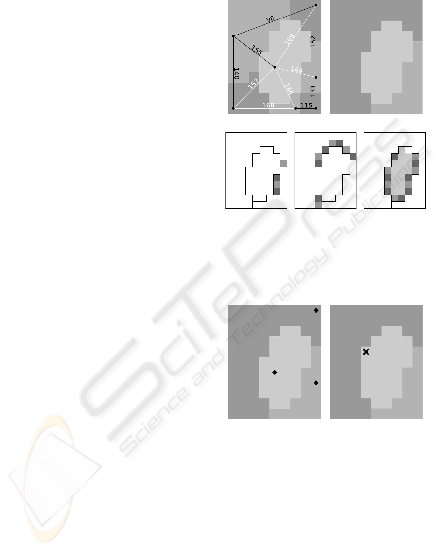
the ROIs as shown in Figure 1. This figure shows the
NRRRs of each ROI. Recall that M
0
must include at
least one pixel of each NRRR.
In contrast, the markers M computed on the RAG
tend to be compact and located more at the center
of each ROI, making them more suitable for user
edition. In Figure 2(a) we show the markers com-
puted on the RAG for the same partition of Figure
1(b). However, if markers M computed on the RAG
are considered on the PAG G
I
, the resulting parti-
tion P
0
= IFT -W S(G
I
, M) may differ from the orig-
inal partition P, as shown in Figure 2(b).
Experimentally, we have observed that the differ-
ences between the original partition P and the recov-
ered one P
0
are located close to the borders. This ev-
idence made us to conjecture that differences are lo-
cated in the tie-zone. In fact, it can be show that P
(the partition selected in the hierarchy) is also an op-
timal solution of IFT -W S(G
I
, M). This implies that
the differences between P and P
0
necessarily belongs
to the tie-zone TZ-W S(G
I
, M). The proof is presented
in the following proposition.
Lemma 1. For any path π
RAG
= hCB
1
,CB
2
, . . . ,CB
n
i
in the RAG of I there is a path π
PAG
=
(a) RAG (b) Selected partition P
(c) 4 NRRRs (d) 9 NRRRs (e) 14 NRRRs
Figure 1: NRRRs computed in G
I
are located close to the
border of the ROIs: (a) RAG edges superimposed on the
primitive CBs, where the MST edges are in black. (b) A
partition P, selected on the hierarchy suppressing the edges
with weight greater than 150. (c)-(e) NRRRs of each ROI
of P, computed in G
I
.
(a) Marker set M (b) Obtained partition P
0
Figure 2: Markers computed in the RAG: (a) Markers of the
MSS of P (each ROI has one NRRR, containing all of its
pixels). (b) Partition P
0
obtained by applying the watershed
on the PAG. The difference between P and P
0
is marked
with an x.
hr
1
, . . . , r
2
, . . . , r
n
i with same cost (according to f
max
)
in G
I
, where r
i
is an arbitrary pixel of the regional
minimum of the catchment basin CB
i
.
Proof. For each pair (CB
i
,CB
i+1
) in π
RAG
, consider
(p
i
, p
i
0
), p
i
∈CB
i
and p
i
0
∈CB
i+1
, as the pair of pixels
that determined the weight of the edge that connects
CB
i
to CB
i+1
on the RAG of I (see (1)).
The path π
PAG
is constructed by linking r
i
to r
i+1
,
INTERACTIVE IMAGE SEGMENTATION WITH INTEGRATED USE OF THE MARKERS AND THE
HIERARCHICAL WATERSHED APPROACHES
189
for 1 ≤ i < n, by connecting r
i
to p
i
and r
i+1
to p
i
0
by the non-decreasing paths contained in the SPF ob-
tained by the IFT-WS when all regional minima are
used as markers (classical watershed).
Proposition 1. Let P = {P
1
, P
2
, . . . , P
n
} be a par-
tition of the image I obtained from the hierarchi-
cal watershed. Consider a set of markers M =
{M
1
, M
2
, . . . , M
n
}, computed on the RAG of I, where
M
i
is the marker associated to P
i
, that is, for i =
1, . . . , n:
M
i
⊆ P
i
and M
i
∩ R 6= ∅, ∀R ∈ NRRR(P
i
) (3)
where NRRR(P
i
) denotes the set of non-redundant re-
ceptive regions of P
i
, computed on the RAG of I. Then,
P is an optimal solution of IFT -W S(G
I
, M).
Proof. Let P
0
= {P
0
1
, P
0
2
, . . . , P
0
n
} be an arbitrary op-
timal solution of IFT -W S(G
I
, M). If ∃p such that
λ
α
= L
P
(p) 6= L
P
0
(p) = λ
β
, then it suffices to show
that f
max
(π
∗
(M
α
, p)) = f
max
(π
∗
(M
β
, p)), where M
α
and M
β
are the markers with labels λ
α
and λ
β
, re-
spectively.
Without loss of generality, suppose that α = 1 and
β = 2. From the optimality of P
0
,
f
max
(π
∗
(M
2
, p)) ≤ f
max
(π
∗
(M
1
, p)). (4)
The MSS is computed in such a way that there is
no tie-zone, which implies that:
f
max
(π
∗
(M
i
,CB)) < f
max
(π
∗
(M
j
,CB)), (5)
i 6= j, ∀CB ∈ P
i
In particular, denoting by V the CB to which p be-
longs,
f
max
(π
∗
(M
1
,V )) < f
max
(π
∗
(M
2
,V )). (6)
From Lemma 1 it follows that:
f
max
(π
∗
(M
i
,V )) = f
max
(π
∗
(M
i
, r
V
)) (7)
From (7) and (6), we have that:
f
max
(π
∗
(M
1
, r
V
)) < f
max
(π
∗
(M
2
, r
V
)) (8)
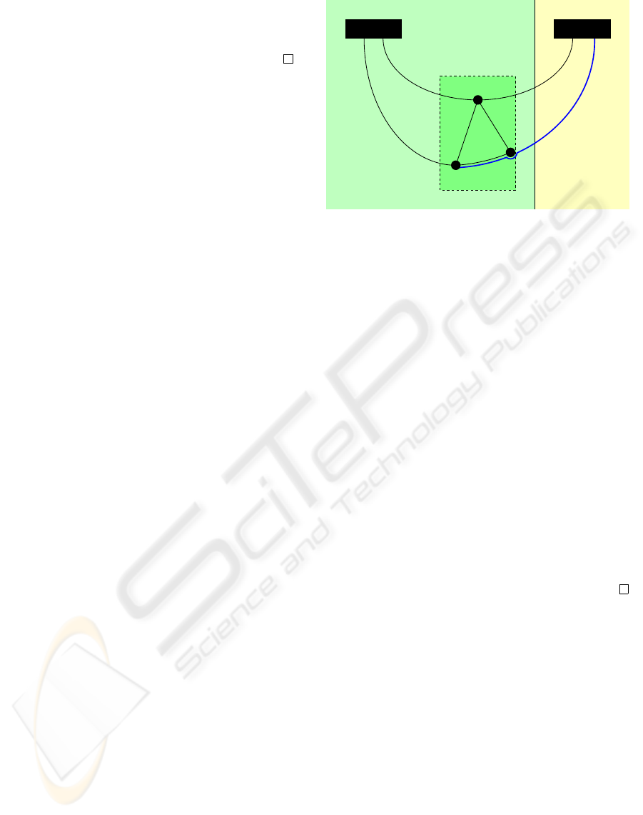
Let v
1
be the first pixel of V in π
∗
(M
2
, p) (see Figure
3). By the choice of v
1
:
f
max
(π
∗
(M
2
, p)) (9)
= f
max
(π
∗
(M
2
, v
1
) ·π
∗
(v
1
, p))
= max{ f
max
(π
∗
(M
2
, v
1
)), f
max
(π
∗
(v
1
, p))}
= max{ f
max
(π
∗
(M
2
, v
1
)), f
max
(π
∗
(v
1
, r
V
)),
f
max
(π
∗
(r
V
, p))}
= max{ f
max
(π
∗
(M
2
, v
1
)), f
max
(π
∗
(v
1
, r
V
)), ∇(p)}
= max{ f
max
(π
∗
(M
2
, r
V
)), ∇(p)}
M
1
P
1
P
2
p
r
V
π
*
(
M
1
,
r
V
)
V
π
*
(
M
2
,
p
)
π
*
(
v
1
,
p
)
v
1
π
*
(
M
2
,
r
V
)
π
*
(
v
1
,
r
V
)
π
*
(
M
1
,
p
)
π
*
(
r
V
,
p
)
M
2
Figure 3: Proof scheme.
As π
∗
(M
1
, p) is an optimum cost path, it follows that:
f
max
(π
∗
(M
1
, p)) (10)
≤ f
max
(π
∗
(M
1
, r
V
) ·π
∗
(r
V
, p))
= max{ f
max
(π
∗
(M
1
, r
V
)), f
max
(π
∗
(r
V
, p))}
= max{ f
max
(π
∗
(M
1
, r
V
)), ∇(p)}
Replacing 8 and 9 in 10:
f
max
(π
∗
(M
1
, p)) (11)
≤ max{ f
max
(π
∗
(M
1
, r
V
)), ∇(p)}
≤ max{ f
max
(π
∗
(M
2
, r
V
)), ∇(p)}
= f
max
(π
∗
(M
2
, p))
Then,
f
max
(π
∗
(M
1
, p)) ≤ f
max
(π
∗
(M
2
, p)) (12)
From 12 and 4, we conclude that
f
max
(π
∗
(M
1
, p)) = f
max
(π
∗
(M
2
, p)). (13)
3.2 From Markers to Hierarchical
Approach
Given a partition P obtained from a set of markers M,
we would like to build an hierarchy that includes P.
In order to do that, two issues need to be considered.
First, as the primitive CBs are considered atomic
in the hierarchy, no partition of the hierarchy con-
tains borders beyond those located at the border of the
primitive CBs. When working with pixel level preci-
sion, if P contains borders that crosses some primitive
CB, then P can not be represented in the hierarchy. If
there are such borders, a possible approach is to set
the same label for all the pixels within each CB, for
example, the most frequent label among them.
Furthermore, it is also necessary that each set of
primitive CBs with same label (that actually make up
VISAPP 2009 - International Conference on Computer Vision Theory and Applications
190
a ROI) is a connected set considering the edges of the
spanning tree of the RAG from which the hierarchy is
constructed. If this is not true, an hierarchy that in-
cludes the desired partition cannot be built. In order
to accomplish this, instead of considering an arbitrary
MST of the RAG, we derive a spanning tree (not nec-
essarily an MST) of the RAG in the following man-
ner:
1. consider an MST for each ROI (set of primitive
CBs with same label), obtaining a spanning forest
of the RAG;
2. complete the spanning forest with edges of mini-
mum weight among the edges of the RAG not yet
used, obtaining a spanning tree of the RAG.
When constructing the TCL, instead of using
all the edges of the spanning tree ordered by their
weights, the edges of the spanning forest obtained at
the first step must be used before the edges added at
the second step.
4 INTERACTIVE
SEGMENTATION TOOL
In this section we describe an interactive segmenta-
tion tool that allows switching back and forth between
the two watershed approaches based on the transitions
described in the previous section. Examples illustrat-
ing the use of these transitions in conjunction with
interaction possibilities from both approaches are pre-
sented.
4.1 Interaction Possibilities
1. Construction of hierarchy of partitions using
uniform flooding or synchronous flooding, with
the following criteria:
• depth (ranking regions by their contrast)
• area (ranking regions by their size)
• volume (ranking regions by their contrast and
size)
The user can navigate through the hierarchy using
a slider control that selects a threshold value for
the weight of the edges to be suppressed in the
hierarchy.
As the selection of a threshold value affects the
entire partition, two local operations (merge and
refine) can be used on the hierarchy to affect only
a desired region of the current partition, as illus-
trated in a simplified hierarchy in Figure 4.
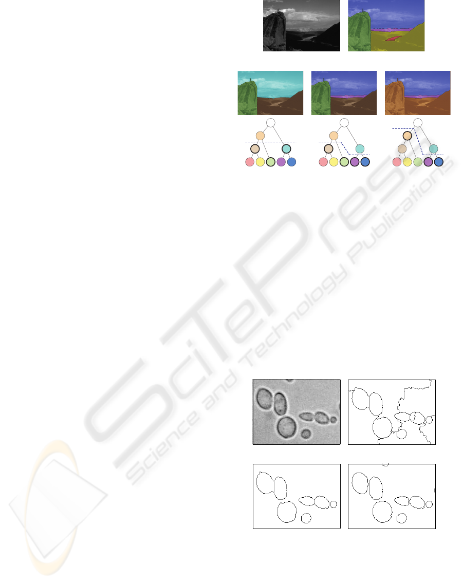
(a) Original image
C
E
D
A
B
(b) Finest partition
F
C
G
A B C D E
F
H
G
I
(c)
F
C
E
D
A B C D E
F
H
G
I
(d)
E
H
D
A B C D E
F
H
G
I
(e)
Figure 4: Obtaining partitions navigating through the TCL:
(c) 3 regions (F, C e G) selected by a threshold value.
(d) Region G split in D and E. (e) Regions F and C merged
in H.
Note that the selection of the threshold value and
the local operations are done on the RAG. Once
the hierarchy is constructed, these operations are
executed in user real time.
2. Automatic generation of markers to partitions
selected from the hierarchy, as described in Fig-
ure 3.1. After switching from the hierarchy to the
markers approach, the user can refine the partition
at a pixel level precision. For example, to separate
cells as shown in Figure 5(d).
(a) (b)
(c) (d)
Figure 5: Segmenting using hierarchy and markers:
(a) Original image. (b) Partition selected on the hierarchy.
(c) Partition after welding regions. (d) Partition with refine-
ments at pixel level precision.
3. Edition of markers using a brush/erase tool.
The labeling function for the markers is derived
associating a unique label for each connected
INTERACTIVE IMAGE SEGMENTATION WITH INTEGRATED USE OF THE MARKERS AND THE
HIERARCHICAL WATERSHED APPROACHES
191
component drawn (for this reason, the user does
not need to change the brush color when marking
each ROI). If markers for distinct ROIs need to be
placed adjacently, the user can use different col-
ors in order to make the markers receive different
labels. The brush and the erase tool are available
selecting only one icon, so the user can edit (draw
and erase) markers just using different mouse but-
tons.
4. Merging of adjacent regions with a welding
brush. This is more flexible than the local merge
operation over the hierarchy, since it can weld re-
gions using edges that are not in an MST of the
RAG, as described in Section 3.2. To accomplish
this, a partition with the selected regions welded
is derived (associating the same label to them) and
this partition is utilized to compute markers or
to derive a hierarchy that contains it (depending
on the approach being used). This operation was
used to obtain the partition shown in Figure 5(c),
as it cannot be found in the original hierarchies
(from the uniform and synchronous floodings).
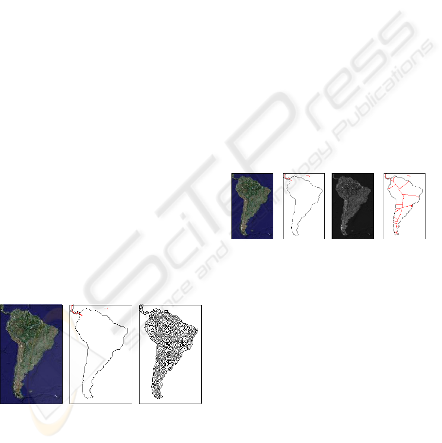
5. Use of the hierarchy in a selected region. This
enables the user to refine a region obtained from
a previous use of the hierarchical watershed, or
from manually created/edited markers. For in-
stance, to obtain the primitive CBs of the land in
a satellite image like the one shown in Figure 6,
one could first design markers by hand in order
to separate land from water, and then select the
finest partition after applying the hierarchy in the
land region. This is a more straightforward way
to achieve the desired partition, instead of first ob-
taining the classical watershed partition for the en-
tire image and them merging all the regions that
are not located at land.
(a) Original image
with markers
(b) Intermediary
step
(c) Desired parti-
tion
Figure 6: Using the hierarchy restricted to a region:
(a) Original image. (b) Partition (with markers) separating
land from water. (c) Primitive CBs of the land region.
4.2 Additional Features
The implemented tool also includes additional fea-
tures:
• Segment automatically option, that executes the
algorithm at each edition of the markers (it can be
disabled to improve performance when designing
markers to segment large images, for instance);
• save the markers image for posterior refinements;
• control over the output image (the user can choose
which images will be superimposed: original im-
age, gradient image, catchment basins, markers
and watershed lines).
• support for segmentation of color images using
the weighted gradient, as described in (Flores
et al., 2004). The user can use either the automat-
ically computed weights or arbitrary weights for
each gradient considered (the weighted gradient
consists in a weighted sum of gradients defined
on each band of the image: hue, saturation and
brightness). The color information can be a key
factor in reducing the interaction effort to obtain a
desired partition, as can be observed in Figure 7.
(a) (b) (c) (d)
Figure 7: Color information reducing the interaction effort
(markers in red, watershed lines in black): (a)-(b) Simple
markers are enough to divide land from water using the
weighted gradient. (c)-(d) Complex markers are needed
when using the morphological gradient of the image ob-
tained without color information.
4.3 A Coarse to Fine Approach
Since markers obtained by computing the MSS on G
I
tend to be located at the borders of the ROIs, they
are not interesting for user edition. Thus, we choose
markers from the MSS computed on the RAG, inde-
pendently of the precision level of the graph being
utilized in the markers approach. With this choice,
the partition obtained by switching from the hierar-
chy to markers over a PAG may differ slightly from
the partition before the switching. Similarly, as noted
in Section 3.2, there may be differences in the inverse
mapping.
Since fine refinements done at a pixel level preci-
sion may be undone by a transition to the hierarchical
VISAPP 2009 - International Conference on Computer Vision Theory and Applications
192

approach or to the region level precision, segmenta-
tion process should follow a coarse to fine approach:
first the user can work with both approaches to obtain
a partition as close as possible to the desired partition,
using only the RAG (which implies efficient process-
ing time); then, using only markers (i.e., editing mark-
ers) over the PAG, he/she can refine the partition at a
pixel level precision.
5 CONCLUSIONS
We investigated how to perform transitions between
the hierarchical and the watershed from markers ap-
proaches. In particular, we discussed the effects ob-
served when these transitions involve changes in the
precision level of the partitions (pixels or regions).
These transitions have been implemented in conjunc-
tion with several interaction possibilities from both
watershed approaches as an interactive segmentation
tool. The implemented tool allows one to take advan-
tage of the best features of each approach and it is ex-
pected that the interaction effort necessary to produce
a desired result may be reduced.
An interesting characteristic of the proposed ap-
proach is that it allows producing partitions with pre-
cisions at pixel or region levels. As a consequence,
the tool may be used for different segmentation pur-
poses.
We plan some use case studies, in order to eval-
uate and improve the usability of the developed tool.
This study should take into consideration not only the
available functionalities but also aspects related to the
interaction process. For example, in applications in
which a precise segmentation is important, the inter-
action effort necessary to draw the markers can still
be very intense. It would be interesting if the tool
could provide means to easily place markers, on both
sides of the borders of interest. As an another exam-
ple, support for color image segmentation is currently
rather limited. These aspects, together with others to
be found in the use case studies, will guide our future
investigations.
ACKNOWLEDGEMENTS
This work is supported by CNPq, Brazil.
REFERENCES
Audigier, R. and Lotufo, R. A. (2007). Seed-relative seg-
mentation robustness of watershed and fuzzy connect-
edness approaches. In SIBGRAPI ’07: Proceedings
of the XX Brazilian Symposium on Computer Graph-
ics and Image Processing, pages 61–70, Washington,
DC, USA. IEEE Computer Society.
Audigier, R., Lotufo, R. A., and Couprie, M. (2005). The
tie-zone watershed: Definition, algorithm and applica-
tions. In Proceedings of IEEE International Confer-
ence on Image Processing (ICIP’05), pages 654–657.
Beucher, S. and Meyer, F. (1993). The morphological ap-
proach to segmentation: the watershed transforma-
tion. In Dougherty, E., editor, Mathematical morphol-
ogy in image processing, chapter 12, pages 433–481.
M. Dekker.
Falc
˜
ao, A. X., Stolfi, J., and Lotufo, R. A. (2004). The
image foresting transform: Theory, algorithms, and
applications. IEEE Trans. Pattern Anal. Mach. Intell.,
26(1):19–29.
Flores, F. C., Polidorio, A. M., and Lotufo, R. A. (2004).
Color image gradients for morphological segmenta-
tion: The weighted gradient improved by automatic
imposition of weights. In SIBGRAPI ’04: Proceed-
ings of the Computer Graphics and Image Processing,
XVII Brazilian Symposium, pages 146–153, Washing-
ton, DC, USA. IEEE Computer Society.
Hahn, H. K. and Peitgen, H.-O. (2003). IWT - interactive
watershed transform: A hierarchical method for effi-
cient interactive and automated segmentation of mul-
tidimensional gray-scale images. In Medical Imag-
ing 2003: Image Processing. Proceedings of the SPIE,
volume 5032, pages 643–653.
Lotufo, R. A. and Silva, W. (2002). Minimal set of markers
for the watershed. In Talbot, H. and Beare, R., ed-
itors, 6th International Symposium on Mathematical
Morphology, pages 359–368. CSIRO Publications.
Marcotegui, B. and Zanoguera, F. (2002). Image editing
tools based on multi-scale segmentation. In Talbot,
H. and Beare, R., editors, Proceedings of ISMM 2002,
pages 127–135.
Meyer, F. (1996). The dynamics of minima and contours. In
Maragos, P., Schafer, R. W., and Butt, M. A., editors,
Mathematical Morphology and its Applications to Im-
age and Signal Processing, pages 329–336. Kluwer
Academic Publishers.
Meyer, F. (2001a). Hierarchies of partitions and morpholog-
ical segmentation. In Scale-Space ’01: Proceedings
of the Third International Conference on Scale-Space
and Morphology in Computer Vision, pages 161–182,
London, UK. Springer-Verlag.
Meyer, F. (2001b). An overview of morphological segmen-
tation. International Journal of Pattern Recognition
and Artificial Intelligence, 15(7):1089–1118.
Zanoguera, F., Marcotegui, B., and Meyer, F. (1999). A
toolbox for interactive segmentation based on nested
partitions. In Proceedings of the International Con-
ference on Image Processing, volume 1, pages 21–25.
INTERACTIVE IMAGE SEGMENTATION WITH INTEGRATED USE OF THE MARKERS AND THE
HIERARCHICAL WATERSHED APPROACHES
193
