
LABELING HUMAN MOTION SEQUENCES USING GRAPHICAL
MODELS
Jos´e I. G´omez
Dpt. Computer Science, University of Jaen, Campus Las Lagunillas, Jaen, Spain
Manuel J. Mar´ın-Jim´enez, Nicolas P´erez de la Blanca
Dpt. Computing Science and Artificial Intelligence, University of Granada, ETSI Informatica y Telecomunicacion
Granada, Spain
Keywords:
Data labeling, Pose estimation, Graphical models, Human motion.
Abstract:
Graphical models have proved to be very efficient models for labeling image data. In particular, they have
been used to label data samples from human body images. In this paper, the use of graphical models is studied
for human-body landmark localization. Here a new algorithm based on the Branch&Bound methodology,
improving the state of the art, is presented. The initialization stage is defined as a local optimum labeling of the
sample data. An iterative improvement is given on the labeling space in order to reach new graphs with a lower
cost than the current best one. Two branch prune strategies are suggested under a B&B approach in order to
speed up the search: a) the use of heuristics; and b) the use of a node dominance criterion. Experimental results
on human motion databases show that our proposed algorithm behaves better than the classical Dynamic
Programming based approach.
1 INTRODUCTION
In this paper, graphical models based on Decompos-
able Triangulated Graphs (DTG) are used to approach
the human-body landmark localization and tracking
problems. Our approach is based on maximizing the
likelihood of the probabilistic graphical model from a
set of image measurements. Assuming that the object
is present in the image, the localization problem rela-
bels the sample data (image features) as part of the ob-
ject or background. Different approaches have been
proposed to label or match image data using graphi-
cal models (Gold and Rangarajan, 1996), (Grimson,
1990), (Haralick and Shapiro, 1992), (Rangarajan
et al., 1997), (Ullman, 1996). Some of these tech-
niques are very general in the sense that they are ap-
plied on any graphical model. However, these ap-
proaches are difficult to apply on data with a substan-
tial amount of clutter. In (Caelli and Caetano, 2005),
graphical models are favorably compared with tradi-
tional relaxation approaches. Figure 1 broadly shows
the main steps of our approach to label new images
from the learned DTG models. In the case of human
motion labeling, the probability distribution defined
by the learned graphical model, can be used as a con-
straint on the set of allowed graph configurations.
The new contributions of this paper are: i) we in-
troduce a new graph labeling algorithm for the DTG
class that improves the standard dynamic program-
ming strategy; ii) we show how the DTG class is able
to capture the human-body pose from different cam-
eras and to identify the point of view.
1.1 Related Work
The DTG class (Amit and Kong, 1996) is introduced
as a simpler graph class to register deformable pat-
terns on static images. More recently, the same graph-
ical model is used to label human body templates in
tracking problems (Song et al., 2003). In both ap-
proaches, a Dynamic Programming algorithm (DP)
was used as the search strategy to find the best label-
ing from a learned model (Fischler and Elschlager,
1973). In a DTG, each node represents a landmark of
the object with an associated vector of measurements.
Although dynamic programming is a very convenient
technique to learn DTG models from data and also to
label new sample data, this strategy presents three im-
portant drawbacks that are analyzed in depth in sec-
tion 2.2. We propose a new algorithm that overcomes
488
I. Gómez J., J. Marín-Jiménez M. and Pérez de la Blanca N. (2009).
LABELING HUMAN MOTION SEQUENCES USING GRAPHICAL MODELS.
In Proceedings of the Fourth International Conference on Computer Vision Theory and Applications, pages 488-495
DOI: 10.5220/0001795704880495
Copyright
c
SciTePress

a
fedcb
Figure 1: Aim of this work. (a) Learned model from data samples ’Gestures’. (b) Input video frame. (c) Detected sample
points around the person. (d) Input to labeling algorithm. (e) Best graph configuration found for input points and model
’Gestures’. Blue circles represent the points selected by our labeling algorithm. (f) Superimposed graph on input video
frame.
those drawbacks, based on a Branch&Bound (B& B)
strategy.
The search for the best labeling is addressed by the
minimum cost path on the tree of all possible label-
ings. However, the best labeling search problem is a
NP-hard problem. Therefore, we approach the search
by using a B& B strategy with an efficient pruning
criterion on the labeling tree. This labeling space is
explored using a first-in-depth strategy, delaying the
final labeling assignment until a minimum cost so-
lution has been found. Two branch prune strategies
have been suggested under a B&B approach in or-
der to speed up the search: a) the use of heuristics;
and b) the use of a node dominance criterion (Fu-
jino and Fujiwara, 1994), (Ibaraki, 1977), (Yu and
Wah, 1988). Here we use a node dominance criterion
because it best suits our problem. In order to obtain
a worst case efficiency of O(N
3
), the same one us-
ing DP on this problem, we design our algorithm to
get the best trade-off between search time and solu-
tion quality, according to the criterion established in
(Hansen et al., 1997). In the experimental section 4,
we show that our algorithm runs in O(N
2
) in most of
our experiments.
Section 2 summarizes the probability model and
discusses the labeling problem using a DTG model.
Section 3 introduces our proposed labeling algorithm.
Section 4 shows the experimental results using differ-
ent human-body models. Section 5 presents our con-
clusions.
2 LABELING USING A DTG
2.1 The Probability Model
A Decomposed Triangulated Graph (DTG) is a trian-
gle collection where there is a vertex elimination or-
der so that the elimination of each node only affects
one triangle (Figure 2). A greedy algorithm (Song
et al., 2000), (Song et al., 2003) is proposed to es-
timate the probability model associated with a DTG
from image data. Here we follow the notation intro-
duced in (Song et al., 2003). Let S = {S
1
,S
2
,...,S
M
}
be a set of nodes, and let X
Si
, 1 ≤ i ≤ M be the mea-
sure associated to each node. The probability model
of a DTG describes the conditional dependences and
independences of triplets of features associated with
the triangles of the DTG. In this case, the probability
density of the set of nodes is
P(X
S
1
,X
S
2
,...,X
S
M
) = P
B
T
C
T
·
T
∏
t=1
P
A
t
|B
t
C
t
(1)
where S = {A
1
,B
1
,C
1
,A
2
,...,A
T
,B
T
,C
T
};
(A
1
,B
1
,C
1
),(A
2
,B
2
,C
2
),...,(A
T
,B
T
,C
T
) are the
triangles, and (A
1
,A
2
,...,A
T
) is the vertex elim-
ination order. Let χ = { X
1
,X
2
,...,X
N
} be a set
of samples where X
n
= {X
n
S
1
,...,X
n
S
M
}, 1 ≤ n ≤ N
represent the labeled data. We have to find the DTG
G that maximizes the likelihood of the samples,
P(χ|G), where
logP(χ|G) ≃ −N·h(X
B
T
,X
C
T
)−N·
T
∑
t=1
h(X
A
t
|X
B
t
,X
C
t
)
(2)
where h(·) is differential entropy or conditional dif-
ferential entropy (Cover and Thomas, 1991). In
other words, we want to find the best sequence
(A
1
,B
1
,C
1
),(A
2
,B
2
,C
2
),··· ,(A
T
,B
T
,C
T
) that mini-
mizes logP(χ|G).
2.2 Searching for the Best Labeling
The search for the best labeling on a DTG using DP
(Amit and Kong, 1996), (Song et al., 2000) has vari-
ous drawbacks:
A) Using DP the lowest cost node is always selected
as the best candidate in the triangle building process.
The search processis carried out in the vertex elimina-
tion order fixed by the DTG. The label process starts
by searching for the pair of sampled points with the
least entropy and iterates adding new nodes. On each
LABELING HUMAN MOTION SEQUENCES USING GRAPHICAL MODELS
489

Figure 2: Example of DTG model on which the problem of vertex repetition is present. Between brackets the vertex elim-
ination order for the model. (a) The first two triangles are obtained. We do not know yet whether these triangles are going
to be in the same DTG; (b) The problem appears when triangle 3 links triangles 1 and 2 in the same DTG; (c) Wrong DTG
obtained.
new iteration the sample point defining the least en-
tropy triangle is labeled. Obviously, this early node
assignment only allows to explore a very small subset
of the labeling space skipping better optimum solu-
tions.
B) The same vertex (label node) can be associated
with different sample points in the labeling process.
In Figure 2 we show a simple example of a DTG with
six vertexes. Let us assume an image with n candidate
points to be labeled as part of the model, where n ≥ 6.
Let us apply a labeling process using DP (Song et al.,
2000), Figure 2 (a) shows two triangles built in the
first step of the process. It is important to remark that
in the building process of both triangles the label (D)
has been used. Figure 2 (b) shows the time in which
the DP algorithm decides to join both triangles. Only
at this time it is possible to detect the problem. This
imposes a high cost in time since we must go back-
wards and forwards in the labeling process in order to
solve this problem (2 (c)).
C) The DP efficiency lower bound is T·O(N
3
) on
DTG (Amit and Kong, 1996), with N being the num-
ber of sample points and T being the number of tri-
angles. Nevertheless, the DP solution is not the best
possible one for this computational efficiency. In Sec-
tion (4) we show that for most of our experiments it
is possible to improve the DP labeling to O(N
2
). In
addition, on more complex types of graph the lower
bound of DP efficiency decreases linearly with the
size of the greatest clique shown in the graph. This
makes its use on complex graphs very inefficient.
3 ALGORITHM FEP
3.1 General Description
In this section we propose a new algorithm that over-
comes the three drawbacks stated above. Let us as-
sume a DTG model with T triangles and let trian-
gle number T be the base triangle of the model.
The triangle number 1 is then associated to the
first vertex in the elimination order of the model.
In order to define a cost for each base edge on
each triangle and for each full triangle, the entropy
measure associated to the vertexes in each case is
used. In other words, for each triangle t with 1 ≤
t ≤ T, Ψ
t
(X
B
t
,X
C
t
) = −h
t
(X
B
t
,X
C
t
) defines the cost
of the base edge (X
B
t
,X
C
t
), and Ψ
t
(X
A
t
,X
B
t
,X
C
t
) =
−h
t
(X
A
t
,X
B
t
,X
C
t
) + h
t
(X
B
t
,X
C
t
) defines the cost of
adding the vertex X
A
t
to the edge (X
B
t
,X
C
t
) in order
to build the triangle (X
A
t
,X
B
t
,X
C
t
). Our goal is to
find the labeling minimizing the value of logP(χ|G)
as given by equation.2. On each iteration, we use ϒ to
denote the cost of the best DTG so far and Λ the cost
of building the new DTG. Λ < ϒ should of course be
verified in order to proceed with the building process.
Let us assume N sample data (points), our ap-
proach is defined by two basic stages: a) to look for
a first solution; and b) improve the current solution
until efficiency reaches O(N
3
).
3.1.1 Looking for the First Solution
We start by building an ordered list of base edges, us-
ing all the possible pairs of nodes, by increasing value
of their associated cost Ψ
t
(X
B
t
,X
C
t
). Then we expand
each edge associating to it the ordered list of candi-
date nodes also by increasing value of their cost. It-
erating this process recursively and using a heuristic
take-the-first on each expanding list, an initial best so-
lution is obtained. The cost of this initial solution is
the ϒ initial value. The improving stage is defined
from a prune strategy on the full labeling tree.
3.1.2 Iterative Improvement
For each list of candidate nodes to a triangle t we de-
fine a dynamic acceptance threshold, DAT, as a pro-
portional value to the difference in entropy to the cur-
rent best solution, ϒ − Λ, divided by the remaining
number of triangles to fit T − t + 1,
DAT =
ϒ− Λ
T − t + 1
> 0 (3)
VISAPP 2009 - International Conference on Computer Vision Theory and Applications
490
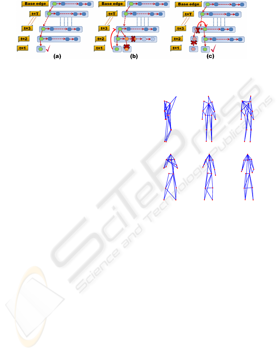
Figure 3: Algorithm FEP: (a) The initial best solution; (b) Searching for a better solution: if a worse DTG is found the
branch is bounded; (c) When a better solution is reached, the best solution is updated. This process is repeated until no
more candidate solutions left or O(N
3
) is reached.
This implies that as the iterative process pro-
gresses, the acceptance threshold for a new node de-
creases, thereby eliminating high cost candidates. Us-
ing the fitting cost and DAT value of the initial solu-
tion we initialize the best fitting cost ϒ and the upper
bound for the DAT value.
The iterative improvement progress from the ini-
tial solution as follows: i) we move two levels up in
the labeling tree (Figure 3 (b)) from the leaf node of
the initial solution; ii) from this new location we try to
build a new solution branching down the second can-
didate of the associated node list (Figure 3(b)); iii) if
the DAT value of the current node is lower than the
upper bound for DAT, we move down first-in-depth
adding the current node to the labeling; iv) we iter-
ate again on the new node, using the same decision
criteria until we reach a leaf node or the DAT value
in the new node has a higher value than the DAT up-
per bound. On each leaf node we calculate ϒ− Λ, the
fitting cost difference between the new solution and
the best solution so far. If negative, we accept the
new solution as the best current solution and we up-
date the Λ and DAT upper bound value. Otherwise,
we go up in the labeling tree and branch in breadth in
order to evaluate the next node. If we reach an O(N
3
)
efficiency during the search, we stop the process ac-
cepting as final solution the best current one.
3.2 Computational Complexity
We apply the technique proposed in (Hansen et al.,
1997) to convert any heuristic search algorithm into
an anytime algorithm offering a trade-off between
search time and solution quality. In the fitting of
a DTG using DP the computational complexity is
always O(T · N
3
) because the number of evaluated
nodes is NMAX
DP
= T · N · (N − 1) · (N − 2) (see
(Amit and Kong, 1996), (Song et al., 2003)). Here
we assume, without loss of generality, that the num-
ber of triangles of the DTG is T > 2, and the num-
ber of points on each frame is N > 6 . In this con-
H(13)
N(14)
LS(11)
RS(1)
LE(10)
RE(7)
LW(9)
RW(6)
LH(8) RH(12)
LK(4)
RK(5)
LA(2)
RA(3)
H(3)
N(11)
LS(13)
RS(1)
LE(14)
RE(8)
LW(12)
RW(7)
LH(10)
RH(9)
LK(5)
RK(6)
LA(2)
RA(4)
H(4)
N(13)
LS(14)
RS(1)
LE(12)
RE(8)
LW(11)
RW(7)
LH(9)
RH(10)
LK(5)
RK(6)
LA(2)
RA(3)
(c)
(b)
(a)
H(12)
N(10)
LS(14)
RS(11)
LE(13)
RE(3)
LW(1)
RW(2)
LH(4)
RH(9)
LK(6)
RK(8)
LA(5)
RA(7)
H(11)
N(10)
LS(8)
RS(9)
LE(3)
RE(4)
LW(1)
RW(2)
LH(5)
RH(12)
LK(13)
RK(7)
LA(14)
RA(6)
H(8)
N(5)
LS(6)
RS(7)
LE(4)
RE(3)
LW(2)
RW(1)
LH(13)
RH(12)
LK(14)
RK(10)
LA(11)
RA(9)
(e)
(f)
(d)
Figure 4: Caltech database (top row): Human DTG models
for several points of view: (a) 0, (b) π/2, (c) π/4. Hu-
manEva database (bottom row): frontal models for differ-
ent actions: (d) Boxing, (e) Gestures and (f) ThrowCatch.
In brackets, vertex elimination order for each DTG. In all
cases N = 14 and T = 12.
text, N
3
< NMAX
DP
. In FEP we set NMAX
DP
as the
maximum number of nodes to evaluate, stopping the
algorithm when this value is reached. We take into
account the number of evaluated nodes in order to fix
the actual efficiency achieved by FEP on each exper-
iment. Our experiments show that a best case com-
plexity of Ω(N
2
) can be reached.
4 EXPERIMENTS ON HUMAN
LANDMARK LABELING
We have tested the performance of the FEP algo-
rithm by carrying out different types of experiments.
Firstly, we have learned human-body models using
static and motion information in order to evaluate the
fitted models. Secondly, we have tested the FEP per-
LABELING HUMAN MOTION SEQUENCES USING GRAPHICAL MODELS
491

formancein order to discriminate among several mod-
els the best one representing a given set of sample
points. In all the cases, we assume that the measure
vector of the nodes follows a multivariate Gaussian
distribution, which substantially simplifies the evalu-
ation of the score measure given by equation (2) (see
(Song et al., 2003)).
4.1 Database Description
We have used two different databases. The Caltech‘s
Database (courtesy of C. Fanti), provides 3D infor-
mation on a set of human-body landmarks in mo-
tion (Fanti et al., 2003). This database contains 3500
samples containing 3D information (position and ve-
locity) of 14 fixed landmarks on a walking human
body: head (H), neck (N), shoulders (LS,RS), el-
bows (LE,RE), wrists (LW,RW), hips (LH,RH), knees
(LK,RK) and ankles (LA,RA). Experiments from dif-
ferent points of view, 0, π/4, π/2, 3π/4 and π radi-
ans, have been conducted using the 3D information.
In order to carry out experiments with more complex
motions, we have also used some actions from the
HumanEva database (Sigal and Black, 2006). The
HumanEva database contains 4 actors performing a
set of 6 actions each one in 3 separate trials. Here
we focus on three of these actions: Box, Gesture and
ThrowCatch. This database provides images from
seven points of view: frontal view (camera C1), lat-
eral views (C2 and C3), and 4 diagonal views (BW1,
BW2, BW3 and BW4).
4.2 Labeling Experiments
The DTG models used in our experiments have been
learned using the algorithm proposed in (Song et al.,
2001). The labeling of a sample is considered cor-
rect if its cost is lower than the true cost assumed as
known (only for the test samples). This criterion un-
fortunately does not guarantee that the fitted labeling
is equal to the true one. The ambiguity defined by
the relative location of the feet in a walking person
seen from the side is impossible to solve by using this
model, and this configuration will have an equal or
lower cost than the true labeling. Also background
points can be selected as part of the best labeling.
4.2.1 Caltech‘s Database
We have used 2500 image samples for learning the
DTG models and 1000 for the labeling experiments.
We learn two different types of models: a) static mod-
els, using only the projections of the 3D positions;
b) motion models, using both the position and veloc-
ity projections. Some of the fitted models from this
(b)
(c)
(d)
(e)
(f)
(a)
Figure 5: FEP working over two samples with 34 points
(14+20): the first sample (a, b, c) shows a π/2 radians point
of view where selected and expected points are coincident;
the second sample (d, e, f) shows a 0 radians point of view
where the points of both legs are exchanged; the remain-
ing body points are fitted correctly. All the points in each
sample are shown in (a) and (d); the points selected by FEP
are shown in (b) and (e); finally, (c) and (f) show the fitted
DTG. Green points: expected and selected labels are coinci-
dents; red diamonds: selected labels are not coincident with
expected labels; blue squares: expected labels that are not
coincident with selected labels.
database are shown in Figure 4 (a)-(c). Once the mod-
els have been learned we use them to label the remain-
ing 1000 samples.
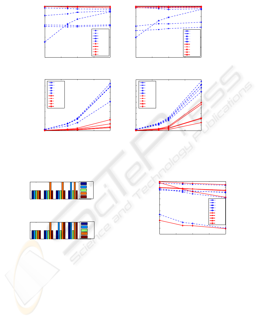
To compare the FEP and DP robustness under
added noise, we run experiments with 14, 20 and 40
random added points over the original 14 points using
the learned static and motion models. In Figure 6 (a)
and (b), the results of both experiments are shown. It
can be observed that in general FEP outperforms DP.
Moreover, the percentage of samples with a labeling
cost equal or lower than the original model is almost
100% for the FEP algorithm in all cases. Only for the
samples in 3π/4 angle do we have 97.8%. Moreover,
in most of the experiments, FEP has O(N
2
) efficiency;
only for angles π/4 and 3π/4 does it reaches O(N
3
)
in certain tests with added noisy points (see Figure 7).
In figure 6 (c) and (d) a comparison on the timing effi-
ciency of both techniques, FEP and DP, using the two
models is shown. In all the cases, FEP outperforms
DP.
It is not an easy task to establish a relationship
between the set of graphs evaluated by FEP and DP
respectively. The main difficulty is in the way the
graph is built. DP starts from the first vertex accord-
ing to vertex elimination order, while FEP starts from
the base triangle, so that the first vertex in DP is the
last added vertex in FEP. In order to assess the qual-
ity of the fitted graph given by DP and FEP, we run
experiments on the Caltech’s database counting the
selected number of correct nodes by each algorithm.
Figure 8 shows the obtained results using the mo-
tion model where both techniques provide equivalent
performance. Results are very similar for the static
model, so only motion model is shown in Figure 8.
VISAPP 2009 - International Conference on Computer Vision Theory and Applications
492
FEPvsDP FEPvsDP
0 10 20 30 40
0
0.2
0.4
0.6
0.8
1
Noisy Points
Correct assignment rate
Motion Model
DP 0
DP pi
DP pi/2
DP 3*pi/4
DP pi/4
FEP 0
FEP pi
FEP pi/2
FEP 3*pi/4
FEP pi/4
0 10 20 30 40
0
0.2
0.4
0.6
0.8
1
Noisy Points
Correct assignment rate
Static Model
DP 0
DP pi
DP pi/2
DP 3*pi/4
DP pi/4
FEP 0
FEP pi
FEP pi/2
FEP 3*pi/4
FEP pi/4
(a) (b)
0 10 20 30 40
0
0.5
1
1.5
2
2.5
3
3.5
4
x 10
4
Noisy Points
Time per frame (ms)
Motion Model
DP 0
DP pi
DP pi/2
DP 3*pi/4
DP pi/4
FEP 0
FEP pi
FEP pi/2
FEP 3*pi/4
FEP pi/4
0 10 20 30 40
0
0.5
1
1.5
2
2.5
3
3.5
4
4.5
x 10
4
Noisy Points
Time per frame (ms)
Static Model
DP 0
DP pi
DP pi/2
DP 3*pi/4
DP pi/4
FEP 0
FEP pi
FEP pi/2
FEP 3*pi/4
FEP pi/4
(c) (d)
Figure 6: FEP versus DP: (a) and (b) performance measured in fitting cost, (c) and (d) timing per frame of FEP and DP
respectively for two models, several angles and different number of noisy points added to the 14 labels used in our models
(Figure 4).
0 14 20 40
O(N)
O(N^2)
O(N^3)
Noisy Points
Efficiency
Motion Model
0
pi/4
pi/2
3pi/4
4pi/4
(a)
0 14 20 40
O(N)
O(N^2)
O(N^3)
Noisy Points
Efficiency
Static Model
0
pi/4
pi/2
3pi/4
4pi/4
(b)
Figure 7: FEP computational complexity: (a) using motion
information; (b) without using motion information. Mea-
sured on tests shown in Figure 6.
4.2.2 HumanEva
For this database the same fourteen landmarks have
been used. Between 6000 and 8000 image samples
of the trial-3 of each action have been used for learn-
ing the DTG models. The only information used dur-
ing the learning process is the projection of the true
3D coordinates of the selected landmark points on
each actor. The 3D coordinates of the landmarks have
been calculated from the information provided with
0 10 20 30 40
0.1
0.2
0.3
0.4
0.5
0.6
0.7
0.8
0.9
1
Noisy Points
Correct assignment rate
Motion Model
DP 0
DP pi
DP pi/2
DP 3*pi/4
DP pi/4
FEP 0
FEP pi
FEP pi/2
FEP 3*pi/4
FEP pi/4
Figure 8: FEPvsDP: Ratio of correct labels using motion
information.
the database. Models for the points of view associated
to cameras C1, C2 and C3 have been learned. Figure
4(d)-(f) shows the learned frontal models for the cam-
era C1. For the testing stage, about 1000 new image
samples from trial-1, for each one of the actions and
cameras, have been used. In this case the data sam-
ples have been generated projecting the full set of 3D
landmark points provided by HumanEva(around 190)
and selecting those projections inside a bounding box
centered on each landmark projection. In average we
obtained between 70 and 100 noisy points per sam-
ple, always including the fourteen landmarks of our
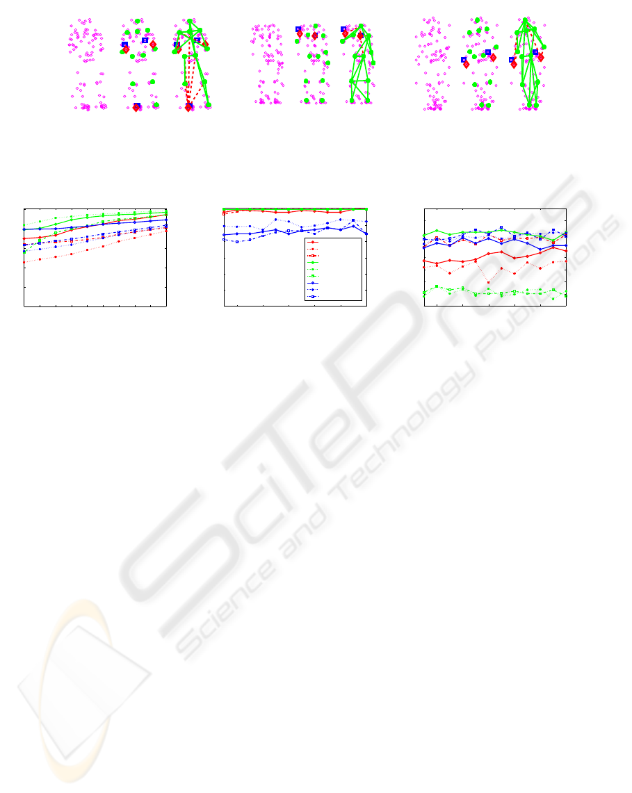
model. Figure 9 (a) shows labeling examples on data
LABELING HUMAN MOTION SEQUENCES USING GRAPHICAL MODELS
493
(b)
(c)
(a)
Figure 9: FEP working on HumanEva samples: (a) Box; (b) Gesture; (c) ThrowCatch. In all cases 14 landmarks and about
70-100 noisy points are used. See Figure 5 for color explanation.
1 2 3 4 5 6 7 8 9 10
0
0.2
0.4
0.6
0.8
1
Accepted distance error in percentage
Correct assignment rate
Ratio of correct assignment labels
2 4 6 8 10 12
0.4
0.5
0.6
0.7
0.8
0.9
1
Block size
Correct assignment rate
Selection of Right Camera
Box_C1
Box_C2
Box_C3
Gestures_C1
Gestures_C2
Gestures_C3
ThrowCatch_C1
ThrowCatch_C2
ThrowCatch_C3
2 4 6 8 10 12
0.2
0.3
0.4
0.5
0.6
0.7
0.8
0.9
1
Block size
Correct assignment rate
Selection of Right Action
(a) (b) (c)
Figure 10: Results on HumanEva database: 9 different models combining actions and points of view are evaluated. In all
cases the actor-1 was selected.(a) Ratio of correct assigned labels according to the distance to its ground-truth landmark.(b)
Ratio of correct detected camera. Each sequence is evaluated with the 3 models associated to its own point of view against
the remaining 6 models. Consecutive windows from 1 to 12 frames are classified on each decision. (c) Ratio of correct
detected actions: the evaluation is performed using the 3 models associated to each action against the remaining 6 models.
from HumanEva using FEP.
Figure 10 (a) shows the FEP performance in se-
lecting the ground-truth labels on each frame. In this
experiment a labeled point is considered correct if its
distance to the ground-truth landmark is less than a
threshold in the range [1-10]% of the actor height.
The best ratio is reached for the Gestures action.
4.3 Point of View and Action
Discrimination
Regarding the application of DTG model in human-
body tracking or motion capture applications, an im-
portant point is to select on each instant the best
model according to the camera point of view. Experi-
ments on HumanEva sequences have been conducted
to evaluate the FEP capability on this task. Figure 10
(b) shows the FEP performance recognizing the right
point of view model. It is remarkable that using a
so simple scheme our results are very encouraging.
In the worst case, the ratio of successful detection is
greater than 80%. We have also conducted experi-
ments on action recognition. Figure 10 (c) shows the
capability of FEP to discriminate one action among
several ones by choosing the model with the best fit-
ting score. Obviously this problem is much more dif-
ficult that the previous one due to the high motion
variability present on each action.In this experiment
our aim is to recognize the action which is performed
in blocks of different number of frames (ranging from
1 to 12 frames). We evaluate different DTG models
on each frame in the target block. A majority vote
scheme is finally used to assign an action class to
each block. In this task, most of the test are above
70% of success and only for Gestures we have a score
of 30%. This is well explained because the Gesture
movements are so general that most of them are in-
cluded as part of the other actions.
5 CONCLUSIONS
We have proposed a new algorithm (FEP), based on
DTG models, which is able to find an optimal label-
ing on human motion data. Experiments have been
carried out using two different databases: Caltech and
HumanEva. It has been shown that on the Caltech‘s
database the FEP algorithm is superior to the tradi-
tional DP algorithm both in terms of efficiency and
quality of the found solution, in spite of its simplic-
ity. The proposed approach could be generalized to
deal with graphical models of higher complexity. This
VISAPP 2009 - International Conference on Computer Vision Theory and Applications
494

point is the subject of forthcoming research.
ACKNOWLEDGEMENTS
This work was supported by the Spanish Ministry
of Science and Innovation under projects TIN2005-
01665 and Consolider Ingenio-2010 (MIPRCV).
REFERENCES
Amit, Y. and Kong, A. (1996). Graphical templates for
model registration. IEEE PAMI, 18(3):225–236.
Caelli, T. and Caetano, T. S. (2005). Graphical models
for graph matching: Approximate models and optimal
algorithms. Pattern Recognition Letters, 26(3):339–
346.
Cover, T. and Thomas, J. (1991). Elements of Information
Theory. John Wiley and Sons.
Fanti, C., Polito, M., and Perona, P. (2003). An improved
scheme for detection and labelling johanson displays.
In NIPS.
Fischler, M. A. and Elschlager, R. A. (1973). The repre-
sentation and matching of pictorial structures. IEEE
Trans. Comput., 22(1):67–92.
Fujino, T. and Fujiwara, H. (1994). A method of search
space pruning based on search state dominance. Jour-
nal of Circuits, Systems and Computers, 25(4):1–12.
Gold, S. and Rangarajan, A. (1996). A graduated assign-
ment algorithm for graph matching. IEEE Trans. Pat-
tern Anal. Mach. Intell., 18(4):377–388.
Grimson, W. E. L. (1990). Object recognition by computer:
the role of geometric constraints. MIT Press, Cam-
bridge, MA, USA.
Hansen, E. A., Zilberstein, S., and Danilchenko, V. A.
(1997). Anytime heuristic search: First results. Tech-
nical Report UM-CS-1997-050.
Haralick, R. M. and Shapiro, L. G. (1992). Computer and
Robot Vision. Addison-Wesley Longman Publishing
Co., Inc., Boston, MA, USA.
Ibaraki, T. (1977). The power of dominance relations
in branch-and-bound algorithms. Journal of ACM,
24(2):264–279.
Rangarajan, A., Chui, H., and Bookstein, F. L. (1997). The
softassign procrustes matching algorithm. In IPMI
’97: Proceedings of the 15th International Conference
on Information Processing in Medical Imaging, pages
29–42, London, UK. Springer-Verlag.
Sigal, L. and Black, M. (2006). Humaneva: Synchronized
video and motion capture dataset for evaluation of ar-
ticulated human motion. Technical report, Brown Uni-
versity, Department of Computer Science.
Song, Y., Feng, X., and Perona, P. (2000). Towards detec-
tion of human motion. IEEE Conference on Computer
Vision and Pattern Recognition (CVPR), 1:810–817.
Song, Y., Goncalves, L., and Perona, P. (2001). Learn-
ing probabilistic structure for human motion detec-
tion. IEEE Conference on Computer Vision and Pat-
tern Recognition (CVPR), 2:771–777.
Song, Y., Goncalves, L., and Perona, P. (2003). Unsuper-
vised learning of human motion. IEEE Trans. Patt.
Anal. and Mach. Intell., 25(7):1–14.
Ullman, S. (1996). High-level Vision. MIT Press.
Yu, C. and Wah, B. (1988). Learning dominance relations
in combined search problems. IEEE Transactions on
Software Engineering, 14(8):1155–1175.
LABELING HUMAN MOTION SEQUENCES USING GRAPHICAL MODELS
495
