A HIERARCHICAL 3D CIRCLE DETECTION ALGORITHM

APPLIED IN A GRASPING SCENARIO

Emre Bas¸eski, Dirk Kraft and Norbert Kr

uger

The Maersk Mc-Kinney Moller Institute, University of Southern Denmark

Campusvej 55 DK-5230 Odense M, Odense, Denmark

Keywords:

3D circle detection, Grasping, Stereo vision, Hierarchical representation.

Abstract:

In this work, we address the problem of 3D circle detection in a hierarchical representation which contains

2D and 3D information in the form of multi-modal primitives and their perceptual organizations in terms of

contours. Semantic reasoning on higher levels leads to hypotheses that then become veriﬁed on lower levels by

feedback mechanisms. The effects of uncertainties in visually extracted 3D information can be minimized by

detecting a shape in 2D and calculating its dimensions and location in 3D. Therefore, we use the fact that the

perspective projection of a circle on the image plane is an ellipse and we create 3D circle hypotheses from 2D

ellipses and the planes that they lie on. Afterwards, these hypotheses are veriﬁed in 2D, where the orientation

and location information is more reliable than in 3D. For evaluation purposes, the algorithm is applied in a

robotics application for grasping cylindrical objects.

1 INTRODUCTION

Circles are important structures in machine vision

since they are a common feature for natural and

human-made objects and they provide more informa-

tion than points and lines about the pose of an ob-

ject. In 3D vision, there are various ways of obtain-

ing edge-like 3D entities (sparse stereo) from a stereo

camera setup. Once the sparse stereo data is grouped

with respect to a perceptual organization scheme, cer-

tain structures can be extracted from individual or

combinations of these perceptual groups. Both, in

dense and sparse stereo the correspondence ﬁnding

phase in 3D reconstruction reduces the reliability of

the information. Therefore, while detecting a certain

structure like a 3D circle by using this kind of infor-

mation, one needs to take into account the noise and

uncertainty of the information.

The algorithms that are used to detect 3D circles

can be grouped into three categories. The ﬁrst cat-

egory consists of voting algorithms like the Hough

transform (Duda et al., 2000). Due to the size of

the parameter space, voting algorithms require much

more memory and computational power than other al-

gorithms.

The second category contains analytical algo-

rithms which use the geometric properties of circles

(e.g., (Xavier et al., 2005)). For laser-range data, this

kind of algorithms run fast and are robust because of

the high-reliability of input data. Stereo vision on the

other hand, introduces too many outliers and uncer-

tainties that make the geometrical properties unstable.

The last category involves ﬁtting algorithms. They

are traditionally based on minimizing a cost func-

tion which depends on a distance function that mea-

sures errors between given points and the ﬁtted circle

(Jiang and Cheng, 2005; Chernov and Lesort, 2005;

Shakarji, 1998). The ﬁtting process can be done ei-

ther in 3D or in 2D. If it is done in 2D, the optimal

plane for the given points is calculated and the points

are projected onto that plane. If the ﬁtting is done

in 3D, the minimization starts with an initial estimate

and tries to converge to the optimal circle. However,

to guarantee convergence, a good initialization is re-

quired. This can be done by starting with multiple

initializations, which decreases the computational ef-

ﬁciency drastically. One can reduce the parameter

space as in (Jiang and Cheng, 2005) but the noisy na-

ture of stereo vision data decreases the probability of

convergence. Therefore, although ﬁtting in 2D is a

decoupled solution (plane ﬁtting and curve ﬁtting are

handled separately), it is more advantageous in terms

of efﬁciency and reliability for noisy data.

In this article, an algorithm which is based on ﬁt-

ting in 2D is presented. Note that, the common prac-

tice for such approaches is using only 3D information

496

Baseski E., Kraft D. and Kruger N. (2009).

A HIERARCHICAL 3D CIRCLE DETECTION ALGORITHM APPLIED IN A GRASPING SCENARIO.

In Proceedings of the Fourth International Conference on Computer Vision Theory and Applications, pages 496-502

DOI: 10.5220/0001796004960502

 SciTePress

and its projection onto 2D. The main speciﬁty of our

approach is, instead of using 3D information only, a

hierarchical representation is used which represents

visual information at different levels of semantic (e.g.,

2D versus 3D) as well as different spatial complexity

(local versus global). By that we obtain information

with different levels reliability. Furthermore, there is

a veriﬁcation process, which is also performed using

different levels in the representation hierarchy.

In this work, the hierarchical representation pre-

sented in (Kr

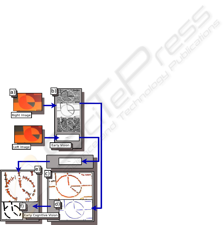
uger et al., 2004) is used. An example

is presented in Figure 1 which shows what kind of

information exists on different levels of the represen-

tation. At the lowest level of the hierarchy, there is

the image with its pixel values (Figure 1(a)). At the

second level, there exists the ﬁltering results (Figure

1(b)) which give rise to the multi-modal 2D primitives

at the third level (Figure 1(c)). At the third level, not

only the 2D primitives but also 2D contours (Figure

1(d)) are available that are created using the percep-

tual organization scheme in (Pugeault et al., 2006).

The last level contains 3D primitives and 3D contours

(Figure 1(e-f)) created from 2D information of the in-

put images.

Figure 1: Different type of information that is available in

the representation hierarchy (a) Original image (b) Filtering

results (c) 2D primitives (d) 2D contours (e) 3D primitives

(f) 3D contours.

Since the reliability and the amount of data de-

creases as the level of the representation hierarchy in-

creases ((Pugeault et al., 2008)), lower levels should

be used to verify the operations done in higher lev-

els. For example, localization of a shape in 3D can be

checked in 2D, once the perspective projection of the

shape is known. Note that, there are more primitives

and their orientation and location information is more

reliable in 2D.

The key idea of our approach is to use differ-

ent aspects of visual information according to their

locality/globality, their semantic richness as well as

their reliability in an efﬁcient way. For example, it is

known that 2D information is more reliable than 3D

(since the stereo correspondence problem introduces

additional errors) but 3D information is required to

ﬁnd 3D position, 3D orientation, and the radius of a

circle. We make use of this trade-off, so that seman-

tic reasoning on a higher level (e.g., 3D information

leads to 3D hypotheses) becomes veriﬁed on a lower

but more reliable level (e.g., 2D information) by feed-

back mechanisms. Another aspect is the locality of

the data being used at the different steps of process-

ing. By using semi-global features (i.e., 2D and 3D

contours) for the computation of hypotheses we de-

crease computational time signiﬁcantly. Since these

hypotheses are veriﬁed using local features, the ef-

fect of additional errors inherent in contours are min-

imized. In this way, we make optimal use of the dif-

ferent levels of the hierarchical representation.

The rest of the article is organized as follows: In

Section 2, the circle detection algorithm is introduced

and some evaluation results in different scenarios with

high variation in terms of circle sizes, 3D positions

and orientation as well as number of circles and other

factors such as occlusion are discussed. The experi-

ments done on different objects in a grasping scenario

where 3D dimension and location play an important

role are presented in Section 3. We conclude with

an evaluation of the algorithm based on these experi-

ments.

2 CIRCLE DETECTION

The algorithm can be summarized in four steps as (1)

ellipse hypotheses creation (Section 2.1), (2) veriﬁ-

cation of these hypotheses (Section 2.2), (3) creating

circles by transferring the veriﬁed hypotheses to 3D

(Section 2.3) and (4) verifying the created circles in

2D (Section 2.4).

A HIERARCHICAL 3D CIRCLE DETECTION ALGORITHM APPLIED IN A GRASPING SCENARIO

497

2.1 Computing Ellipse Hypotheses

Because of the correspondence problem in the 3D re-

construction process, the information in 2D can not

be transferred to 3D completely. Therefore, contours

in 2D contain more primitives than corresponding 3D

contours and a 2D contour can contain projections of

more than one 3D contour. These facts are the moti-

vation to use 2D contours to search for 2D ellipses in

the image. Another important fact is that, a single 2D

contour may not be big enough to compute the ellipse

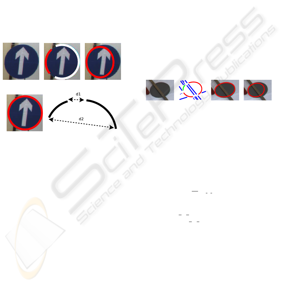
that we are searching for. In Figure 2(c) and (d), the

ellipses ﬁtted to contours in Figure 2(b) are shown.

Since the red contour is not big enough, the ellipse

ﬁtted to that contour is not the desired one.

(a) (b) (c)

(d) (e)

Figure 2: (a) Original image (b) Two contours on the circle

(One is red and the other is white) (c) Fitted ellipse to the

red contour in (b) (d) Fitted ellipse to the white contour in

(b) (e) Two curves can be merged if min(d1,d2) is small

enough.

Having too small data sets for ﬁtting is a com-

mon problem originating from perceptual organiza-

tion. To overcome this difﬁculty, a merging mech-

anism has been proposed in (Ji and Haralick, 1999)

which is based on proximity. Two curve segments

are merged if the distance between their closest end

points is smaller than a certain value (Figure 2(e)).

The ﬁrst step of the algorithm starts with merging the

2D contours by using the proximity criterion. This

merging operation creates a new set of 2D contours

which contain the old 2D contours and their combi-

nations.

Let C

be the set of all 3D contours whose pro-

jections on the image plane are contained in the 2D

contour c

. Then, for the 3D contour C

, P · C

∈ c

iff C

∈ C

(P is the projection matrix). Note that

when two 2D contours are combined, the result is

represented as c

and the set of 3D contours whose

projections on the image plane are contained by the

combination is represented as C

The ellipse hypotheses e

that the 3D circles are

based on are created from the combined contours

where c

is the 2D combined contour to which e

ﬁtted. The ellipse ﬁtting is done using the algorithm

in (Pilu et al., 1996) which is an ellipse speciﬁc least-

squares ﬁtting method. The ﬁtted ellipses are repre-

sented using the general ellipse equation given in (1).

+ 2bxy + cy

+ 2dx + 2 f y + g = 0 (1)

2.2 Veriﬁcation of Ellipse Hypotheses

Since we use the merged contours, the ﬁtting proce-

dure creates a lot of false ellipses as well as true ones.

Therefore, not all the ﬁtted ellipses are really in the

scene. A true ellipse is shown in Figure 3(c) which

is ﬁtted to the combination of the two red contours in

Figure 3(b) and a false ellipse is shown in Figure 3(d)

which is ﬁtted to the combination of the bottom red

and the green contour in Figure 3(b).

(a) (b) (c) (d)

Figure 3: (a) Input image (b) 2D contours (c) A true ellipse

(d) A false ellipse.

The elimination of false ellipses is done by ﬁnd-

ing the signiﬁcance (Lowe, 1987) of the ellipses. The

percentage of covered length of e

is calculated from

all 2D primitives (represented by π

) that satisfy the

following equations:

kπ

− e

k ≤ α

(2)

|arctan(

)

) − θ

| ≤ α

(3)

where α

and α

are thresholds, (2) is the distance

between π

and e

, (3) is the difference between the

slope of e

at (x

) and the orientation of π

(repre-

sented by θ

) and (x

) is the coordinate of the clos-

est point on e

to π

. If π

satisﬁes (2) and (3), its patch

size (the diameter of the patch covered by the primi-

tive) is added to the total covered length of e

. If the

percentage of total covered length of e

with respect

to its perimeter is higher than a threshold, namely α

the ellipse is qualiﬁed as a true ellipse. The true el-

lipses for some scenes are shown in Figure 4 where

= 1 pixel, α

= 10

◦

and α

= 60%.

2.3 Computing 3D Circle Hypotheses

Due to the fact that the perspective projection of a cir-

cle on the image plane is an ellipse, it is possible to

VISAPP 2009 - International Conference on Computer Vision Theory and Applications

498

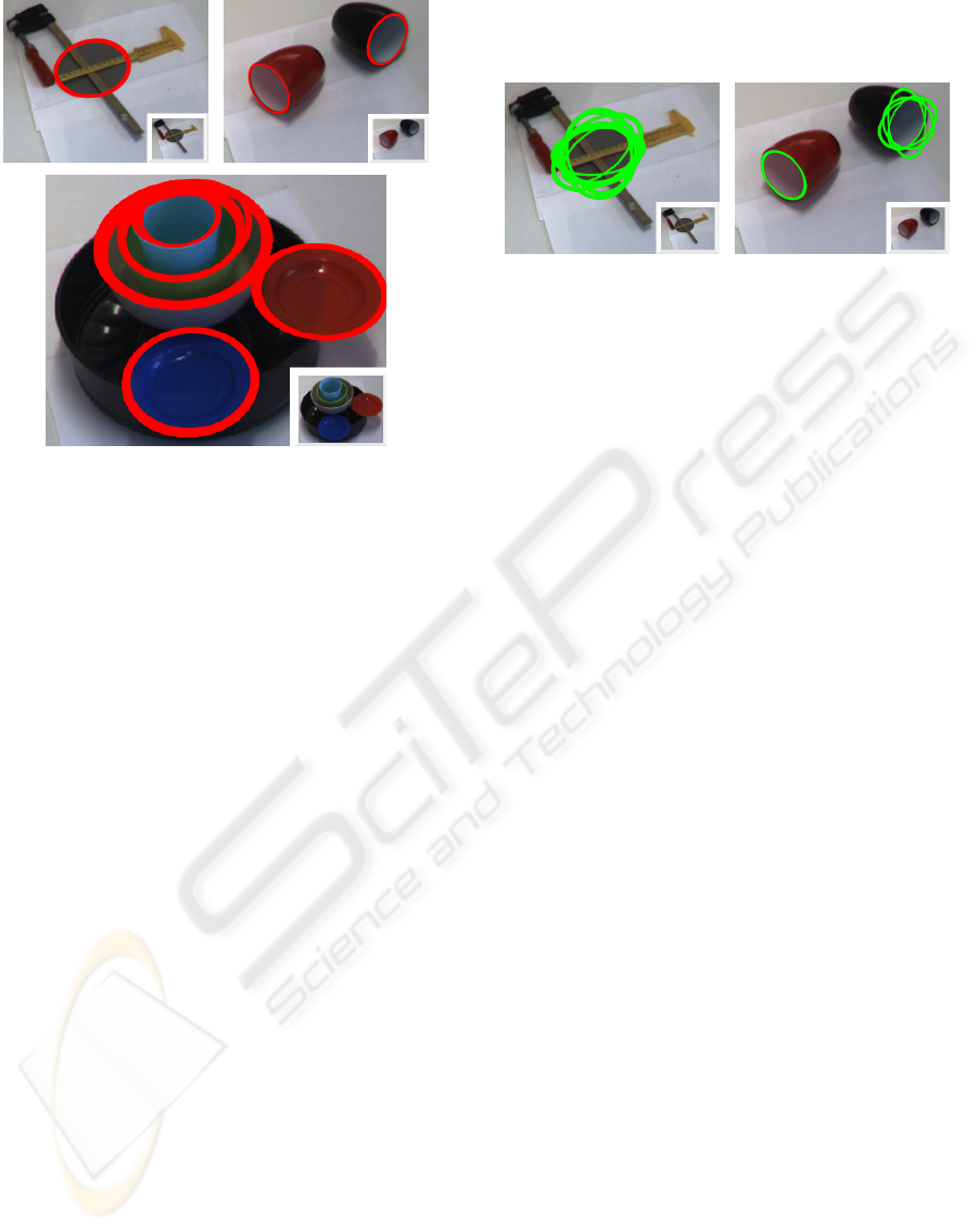
Figure 4: Some true ellipse examples.

reconstruct the 3D circle, once the plane that the cir-

cle lies on is known. Therefore, at this point, to create

3D circles, the only further information we need is the

plane p

on which the circle that will be created from

ellipse e

lies. After calculating p

, camera geometry

can be used to ﬁnd all the parameters of the 3D circle

whose perspective projection is e

. Since we know the

2D contour c

which gave rise to e

, it is possible to

use the 3D contours C

whose projections are con-

tained by c

to ﬁt p

. This operation gives the normal

vector of the 3D circle as it is parallel to the normal

vector of p

. What is missing for the 3D circle is the

center and the radius in 3D.

To ﬁnd the center and the radius of the circle,

discrete points on e

are multiplied with the pseudo-

inverse of the projection matrix (P

) to create rays,

passing through the camera center and the discrete

points of the ellipse. The intersections of these rays

and the ﬁtted plane p

gives 3D points which are sup-

posed to belong to the 3D circle. The center of mass

of these 3D points gives the center of the 3D circle

and this center is used to calculate the radius as the

average distance of the 3D points to the center. Note

that, the 3D circles calculated in the this step can be

represented in parametric form as:

Rcos(t)~u + R sin(t)(~n ×~u) +~c (4)

where ~u is a unit vector from the center of the circle

to any point on the circumference; R is the radius; ~n

is a unit vector perpendicular to the plane and~c is the

center of the circle.

Some results are presented in Figure 5(a-b). Note

that more than one combined contour can represent

the same ellipse and they produce correct circles as

well as false ones because of the 3D reconstruction

uncertainties. The false circles are eliminated in the

next step.

(a) (b)

Figure 5: (a-b) Projection of 3D circles on the image plane

before veriﬁcation.

2.4 Final Selection of Circle Hypotheses

As the last step, our aim is to ﬁnd which 3D circle

is the best for ellipses that have been represented by

more than one combined contour. Let E

be the set

of ellipses that are similar. It is impossible for them

to have the same curve parameters so we can measure

the similarity between two ellipses as a cost function

depending on the distance between their centers, the

difference of their perimeters and orientations. The

main idea of the last step is to calculate the signiﬁ-

cance of ellipses which are projections of circles cre-

ated from the ellipses in set E

. We do the evaluation

in 2D since the amount and the reliability of data in

this dimension is higher than 3D. To ﬁnd the ellipse

which is the perspective projection of a 3D circle, we

can pick 5 points of the circle on the image plane and

use the implicit equation of the conic through 5 points

as in (5).



xy y

x y 1

···



= 0 (5)

The 5 points can be created from (4) for t ∈

{0,80...320}. Equation 5 gives the generic equation

of an ellipse as in (1). Therefore, we ﬁnd the sig-

niﬁcance of these projected ellipses by using all 2D

primitives π

that satisfy Equations (2) and (3). For

each set E

, only the one circle with the highest sig-

niﬁcance is kept. Some results are presented in Figure

6 and 7.

2.5 Problems

Although the algorithm is stable on tilted, partially

occluded and cluttered circles, perceptual organiza-

tion can create problems in case of good continuation

between circular and non-circular parts. Figure 8(b)

A HIERARCHICAL 3D CIRCLE DETECTION ALGORITHM APPLIED IN A GRASPING SCENARIO

499

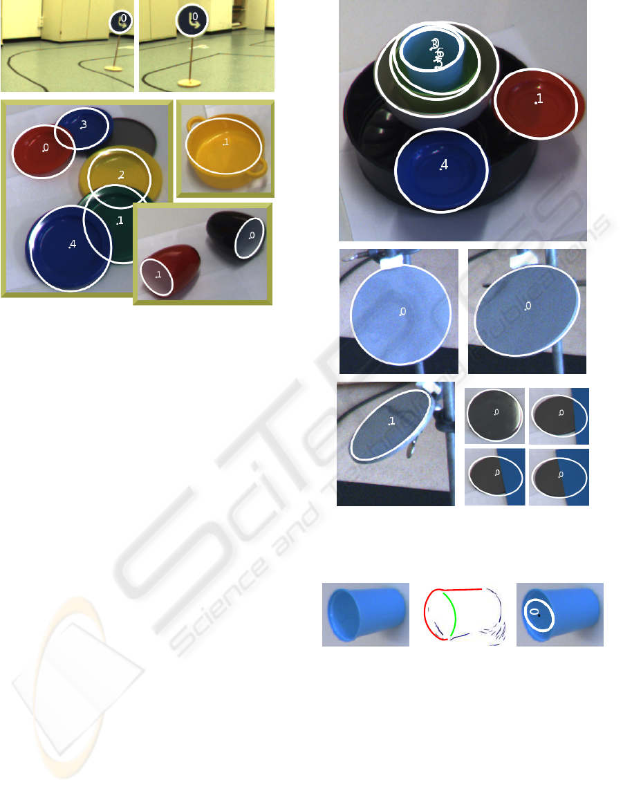
Figure 6: 3D circle detection results on different scenarios.

(White ellipses are the projections of 3D circles onto the

image plane).

illustrates a case, where the red 2D contour combines

a circular and a non-circular part. In such cases, the

remaining circular part (e.g., green contour in Figure

8(b)) may create a valid ellipse hypothesis but trans-

ferring this hypothesis to 3D is heavily dependent on

the plane that is ﬁtted to the 3D points and usually

this situation leads to incorrect 3D circles as shown in

Figure 8(c).

3 APPLICATION IN A GRASPING

SCENARIO

The algorithm described in the previous section is ap-

plied in a robot grasping application. In this section

we describe the setup and use of this application to

evaluate the circle detection.

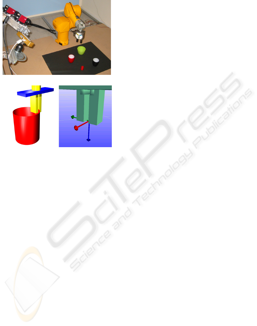
3.1 System Description

The robotic system used consist of a six degree of

freedom industrial robot (St

aubli RX-60B), a two ﬁn-

ger parallel gripper (Schunk PG 70) and a Point Grey

BumbleBee2 stereo camera (see Figure 9(a)). The

camera is calibrated relative to the robot coordinate

system. Therefore the output of the above algorithm

can be directly used for the computation of the grasp-

ing position.

Figure 7: 3D circle detection results for multiple objects,

different orientation and occlusion. (White ellipses are the

projections of 3D circles onto the image plane).

Figure 8: (a) Original image (b) 2D contours corresponding

to (a) (c) Detected 3D circle.

3.2 Grasp Deﬁnition

For this work we selected one of the grasps deﬁned in

the grasping application to evaluate the quality of the

circle detection. The cylindrical object is grasped on

its brim (see Figure 9(b)). The position of the grasp is

expressed similar to the parametric form in (4). From

this observation directly follows that there is actually

not one possible grasp, but a one dimensional mani-

fold of grasps (varying the grasp position around the

VISAPP 2009 - International Conference on Computer Vision Theory and Applications

500

(a)

(b)

(c)

Figure 9: (a) Robot system consisting of six degree of free-

dom industrial robot, two ﬁnger gripper and two stereo cam-

era systems (The lower camera systems was used for this

work). (b) Grasp at the brim of the cylindrical object. (c)

Gripper coordinate system.

circumference of the circle). Additionally the grasp-

ing depth h can be chosen according to the require-

ments of the scene. The position p of the grasper can

therefore be deﬁned as:

~p = Rcos(t)~u + R sin(t)(~n ×~u) +~c −~nh . (6)

Figure 9(c) shows the position and orientation of the

grasper coordinate system deﬁned at the end of the

ﬁngers. The grasper needs to be aligned in the follow-

ing way: ~z

= −~n and ~y

= cos(t)~u + sin(t)(~n ×~u).

While the gripper opening can be deﬁned as d =

min(2R,d

max

3.3 Evaluation

Figure 10 shows a number of scenarios where the

gripper is moved to the grasping position computed

based on the circle information (h = 2 cm, t was used

in a standard conﬁguration except when this would

have lead to a collision). For the set of experiments

shown, the number of true positives (a circle that ex-

ists in the scene is detected) is 35, the number of false

negatives (a circle that exists in the scene is not de-

tected) is 1 and the number of false positives (a cir-

cle is detected that is not present in the scene) is 13.

As a conclusion, 97.2% of the circles present in the

scene have been detected and out of all detected cir-

cles (true positives and false positives), 72.9% of them

correspond to the circles present in the scene. Note

that, the false positives occur for relatively big circles

where the numerical stability decreases. On the other

hand, using the saliency measure (which is high for

true positives) of the found circles, the true positives

have higher chance to be choosen for grasping. Also,

the different setups show that our system is able to

cope with different levels of complexity.

4 CONCLUSIONS

We have discussed a 3D circle detection algorithm

which makes use of different aspects of 2D and 3D in-

formation for hypothesis generation and veriﬁcation.

To be able to cope with the uncertainties of sparse

stereo data, 3D circles are localized in 3D by con-

sidering 2D hypotheses and veriﬁed in 2D, where the

information is more reliable. The potential of the ap-

proach has been shown on a grasping application for

different scenarios. As a future work, the problem of

combining circular and non-circular parts will be han-

dled by splitting 2D contours with respect to junctions

and 3D structure of the contour.

ACKNOWLEDGEMENTS

The work described in this paper was conducted

within the EU Cognitive Systems project PACO-

PLUS (IST-FP6-IP-027657) funded by the European

Commission.

REFERENCES

Chernov, N. and Lesort, C. (2005). Least Squares Fitting of

Circles. J. Math. Imaging Vis., 23(3):239–252.

Duda, R. O., Hart, P. E., and Stork, D. G. (2000). Pattern

Classiﬁcation. Wiley-Interscience Publication.

Ji, Q. and Haralick, R. M. (1999). A Statistically Efﬁcient

Method for Ellipse Detection. In ICIP (2), pages 730–

734.

Jiang, X. and Cheng, D.-C. (2005). Fitting of 3D Circles

and Ellipses Using a Parameter Decomposition Ap-

proach. In 3DIM ’05: Proceedings of the Fifth In-

ternational Conference on 3-D Digital Imaging and

Modeling, pages 103–109. IEEE Computer Society.

uger, N., Lappe, M., and W

org

otter, F. (2004). Bi-

ologically Motivated Multi-modal Processing of Vi-

sual Primitives. The Interdisciplinary Journal of Ar-

A HIERARCHICAL 3D CIRCLE DETECTION ALGORITHM APPLIED IN A GRASPING SCENARIO

501

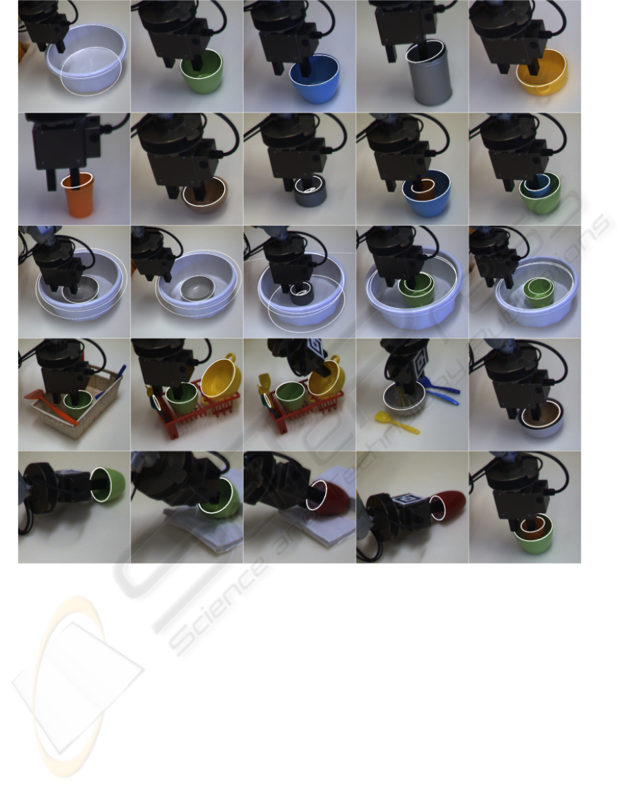
Figure 10: Detected circles and applied grasps. The circles were drawn into the images and the occluded parts were corrected

afterward to improve the readers scene understanding. The scenes are of different complexity, starting out with single objects,

going to objects included in each other, multiple (and more complex) objects and ﬁnally tilted single objects.

tiﬁcial Intelligence and the Simulation of Behaviour,

1(5):417–428.

Lowe, D. G. (1987). Three-Dimensional Object Recogni-

tion from Single Two-Dimensional Images. Artiﬁcial

Intelligence, 31(3):355–395.

Pilu, M., Fitzgibbon, A., and Fisher, R. (1996). Ellipse-

Speciﬁc Direct Least-Square Fitting. In In Proc. IEEE

ICIP.

Pugeault, N., Kalkan, S., Bas¸eski, E., W

org

otter, F., and

uger, N. (2008). Reconstruction Uncertainty and

3D Relations. In Proceedings of Int. Conf. on Com-

puter Vision Theory and Applications (VISAPP’08).

Pugeault, N., W

org

otter, F., and Kr

uger, N. (2006). Multi-

modal Scene Reconstruction Using Perceptual Group-

ing Constraints. In Proceedings of the IEEE Work-

shop on Perceptual Organization in Computer Vision

(in conjunction with CVPR’06).

Shakarji, C. (1998). Least-Squares Fitting Algorithms of

the NIST Algorithm Testing System. Res. Nat. Inst.

Stand. Techn., 103:633–641.

Xavier, J., Pacheco, M., Castro, D., Ruano, A., and Nunes,

U. (2005). Fast Line, Arc/Circle and Leg Detection

from Laser Scan Data in a Player Driver. In Robotics

and Automation, 2005. ICRA 2005. Proceedings of the

2005 IEEE International Conference on, pages 3930–

3935.

VISAPP 2009 - International Conference on Computer Vision Theory and Applications

502