NEW CLOSED FORM SOLUTIONS FOR SKELETAL

EXTRACTION FROM MOTION CAPTURE

Jonathan Kip Knight

ITT, Colorado Springs, U.S.A.

Sudhanshhu Kumar Semwal

Departmemt of Computer Science, University of Colorado, Colorado Springs, U.S.A.

Keywords: Sphere-fit, Motion capture, Skeleton.

Abstract: We present a fast closed form solution for estimating the exact joint locations inside the human body from

motion capture data. The new closed-form solution is more robust and faster. For example, the formulae are

as much as about 100 times faster than the traditional non-linear Maximum Likelihood Estimator and about

9 times faster than linear least squares methods. The methods are proven to be statistically efficient when

measurement error is smaller than the joint-marker distance. Unbiased Generalized Delogne-Kása (UGDK),

multiple radii solution, and incremental GDK are important contributions of our research providing closed

form fast solutions for skeleton extraction from motion capture data. Skeletal animation sequences are

generated using the CMU and Eric Camper’s motion capture database.

1 INTRODUCTION

Skeleton extraction methods use temporal marker

positions from motion capture data to predict the

joint locations. These predicted joint locations then

define the skeleton. Recently, O’Brien et al., in 2000

(Brian, 2000) and with Kirk (Kirk, 2005) have

produced a fast method for skeleton extraction using

a linear least squares method assuming there is a

relatively stationary point between two segments,

and then solving for that point, which is essentially

the rotation point. Some years ago, Leendert de

Witte (Witte, 1960) found a solution for a circle in

3-D space. The Maximum Likelihood Estimator

(MLE) was the first solution for finding the sphere

parameters. In 1961 Stephen Robinson (Robinson,

1967) presented the iterative method of solving the

sphere and developed a closed form solution for the

radius estimator but not for the center estimator. In

1972, Delogne presented (Delogne, 1972) a method

for solving a circle for the purposes of determining

reflection measurements on transmission lines.

István Kása (Kasa, 1976) was the first to recognize

the bias in the answer and produced better error

analysis. Vaughan Pratt (Pratt, 1987) produced a

very generic linear least squares method for

algebraic surfaces. Gander (Gander, 1994) produced

the linear least-squares method for circle fitting.

Samuel Thomas (Thomas, 1995) created a formula

for the Cramér-Rao Lower Bound for the circle

estimation. Lukács (Lukas, 1997) produced some

improvements on non-linear minimization for

spheres. Corral et al. (Corral, 1998) analyzed Kása’s

formula in more detail and a way to reject the

answer if the confinement angle got too small.

Strandlie et al. (Strandlie, 2000) transformed a

Riemann sphere into a plane and fit the plane using

standard methods involving the eigenvalues of the

sample covariance matrix. Zelniker (Zelnicar, 2003)

reformulated the circle equation to solve directly for

the center using the pseudo-inverse (

) of a 2xN

matrix. Michael Burr et al. (Burr, 2004) created a

geometric inversion technique which far surpassed

the complexity needed to solve for a hypersphere.

Knight et al. (Knight, 2007) published the initial

results from the research for this dissertation in

which a skeleton was formed from a closed-form

solution of generic motion capture data.

249

Semwal S. and Knight J.

NEW CLOSED FORM SOLUTIONS FOR SKELETAL EXTRACTION FROM MOTION CAPTURE.

DOI: 10.5220/0001799702490256

In Proceedings of the Fourth International Conference on Computer Graphics Theory and Applications (VISIGRAPP 2009), page

ISBN: 978-989-8111-67-8

2 SKELETAL EXTRACTION

Producing a skeleton involves finding the centers of

joint rotations, the hierarchy of segmentation, and

the orientation of each segment. The hierarchy of

segmentation is known ahead of time such as in

human animation. The orientation of a segment is

determined by one of two methods. Either it is given

in the raw data, e.g. magnetic trackers, or it is

calculated by the fastest technique known. One of

the earliest uses found in motion capture were

published by Herda et al. (Herada, 2000). The most

common approach to calculating a skeleton from

motion capture data is through minimization until

the skeleton fits where the rotation points have been

approximated. The minimization involves squishing

segments and moving joints until all joints are

nearest to the calculated rotation points. O’Brien et

al. (O’Brian, 2000) uses a linear least-squares

minimization that produces the rotation points from

a collection of time frames. In their study, magnetic

motion tracking devices are used which contain both

position and orientation. This is akin to solving for

the best-fit sphere around a center. 3D marker

trajectories are also analyzed in (de-Aguiar, 2006).

In the following section, we start with

explanation of symbols and conventions. In Section

4, we visit some methods which have been used in

various techniques as a prelude to generalized

Generalized Delogne-Kása (GDK) method in

Section 5 which include three contributions of our

paper – unbiased GDK (Section 6), multiple radii

solution (Section 7), and incremental GDK (Section

8). A comparison of all techniques is in Section 10

along with further research (Section 11).

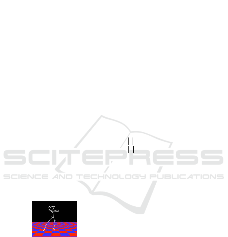
Figure 1: Skeleton from motion capture data.

3 SYMBOLS

(

)

-- on the order of (i.e. size of) y

-- number of measurements

CRLB

-- Cramér-Rao Lower Bound covariance of

estimator

D -- dimension of hypersphere

FLOP

-- floating point operation

--- i

measurement of position

--- average of all measurements of positions

--- expectation of the i

position

--- average of expectations of all positions

-- measurement covariance of each position

-- measurement covariance estimator

-- measurement standard deviation

C -- sample covariance

-- true covariance of expected positions

S -- sample third central vector moment

-- true third central moment of expected positions

F -- true 4th central moment of expected positions

--- center estimator

-- true center of hypersphere

-- radius estimator

-- true radius of hypersphere

-- eigenvalue of matrix

v -- eigenvector of matrix

-- transpose of column vector into row vector

−

-- multiplicative inverse of matrix

-- transpose of matrix

∇

-- vector gradient operator

-- magnitude of vector

-- determinant of matrix

(

)

-- 3D vector Normal Distribution

(

)

-- spectral radius of matrix

Tr A

(

)

-- trace (sum of diagonals) of matrix

(

)

-- expectation of random variate

Var A

(

)

-- variance of random variate

Cov A,B

(

)

-- covariance of two variates

4 SPHERICAL CURVE FITTING

APPROACHES

There are three techniques in use today: iterative;

least squares; and algebraic best fits. They each have

their advantages and disadvantages. Iterative

techniques are good for accuracy, least squares are

faster than iterative but slower than algebraic, and

algebraic techniques are good for speed.

4.1 Monte-Carlo Experiments

In order to compare the methods, a Monte-Carlo

experiment was run using 1000 trials, each of which

had anywhere from 4 to 1,000,000 samples. The

runs took over a week of computational effort to

collect. Each trial had a fixed standard deviation of

the samples from the sphere with values ranging

GRAPP 2009 - International Conference on Computer Graphics Theory and Applications

250

from 10

-13

to 10

. The sample must be confined to

be within an angle from a fixed point on the sphere.

This experiment allows for the in-depth analysis of

the error in the answer from four different

estimators. The four techniques are Maximum-

Likelihood Estimator (MLE) (Section 4.3), Linear

Least-Squares (LLS) (Section 4.4), Generalized

Delogne-Kása Estimator (GDKE) (Section 5), and

the new Unbiased Generalized Delogne-Kása

estimator (UGDK) explained in Section 6. The first

three are established formulae and has been used for

two hundred years (MLE (Shakarji, 1998)) to as

young as three years (GDKE (Zelnicker, 2003)).

UGDK is new method proposed in this paper. The

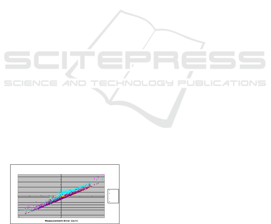
following graph (Figure 2) shows the errors in the

estimators compared to the standard deviation of the

samples indicating that UGDK performs closest to

CRLB. The graph shows that the relative error

versus relative standard deviation is a line for each

of these methods. The error is thus proportional to

the standard deviation on a log-log display showing

a power law. What is also clear from the graph is the

comparison. The outliers on the graph have been

circled. The obvious differences between the

estimators show up in the graph by deviations from

the straight line when error equals standard

deviation. From the graph, it appears that there is a

common limitation to the error in the estimator. This

common limitation is named the Cramér-Rao Lower

Bound to the covariance of an estimator. The

following sections discuss the limit to all estimators

for this particular problem. The MLE has outliers

when the error equals the radius. This is due to

multiple solutions when the error equals the radius.

The LLS has outliers when the standard deviation is

below about 10

-6

times the radius and greater than

times the radius. These are due to numerical

instability during the extremes of using finite

representation of decimal numbers. The GDKE

seems to be on par with the MLE except for the

MLE outliers. The UGDK is consistently close to

the CRLB indicating that it is more accurate than

other methods.

Error of Center Estimate

1E-17

1E-15

1E-13

1E-11

0.000000001

0.0000001

0.00001

0.001

0.1

1000

100000

10000000

1000000000

1E+11

1E+13

1E+15

1E+17

1E-14 1E-10 0.000001 0.01 100 1000000 1E+10 1E+14

MLE

LLS

GDKE

UGDK

CRLB

Figure 2: Shows relative error comparison.

4.2 Cramér-Rao Lower Bound (CRLB)

The Cramér-Rao Lower Bound (CRLB) is the

proven lower bound for any estimator’s covariance.

It is equal to the inverse of the Fisher Information. It

is an important measure when dealing with any

estimator because it is the best error that an

estimator can achieve. All estimators will have at

best an error of the CRLB.

4.3 Non-linear Maximum Likelihood

Estimator (MLE)

According to the National Institute of Standards and

Technology (NIST) (Shakarji, 1998) the best way to

find the center of a sphere is through non-linear

minimization of the variance of the radius. This is

also called the Maximum-Likelihood Estimator

(MLE) for the center

and radius

. The

minimization is usually carried out by iterative

methods like the Levenberg-Marquardt Method

(Shakarji, 1998) and cannot be solved directly.

4.4 Linear Least Square Method (LLS)

The next best thing to the very slow MLE method is

through linear least-squares solution. This is usually

an over-constrained problem since there are N

equations and four (i.e. D+1) unknowns. The N

equations can be put into a single matrix equation to

solve with standard linear algebra techniques. When

LLS and CRLB are compared, once again, the

outlier cases show that the answer erroneously lies

on the sphere. For the most part, the answer error is

proportional to the square root of the CRLB. The

next fastest algorithm is the linear least squares

method which has been analyzed in floating point

operations (FLOPS) in (Knight, 2008) with D=3 as

FLOPs 3

(

)

= N236 + 709

An estimator of a parameter is considered biased

if it is expected to be a little off of the real answer.

Zelniker (Zelnicker, 2003) has shown that the bias of

the GDKE is on the order of the measurement

standard deviation. Our statistical analysis has

shown that there are cases when the bias is quite

significant and does not disappear even when more

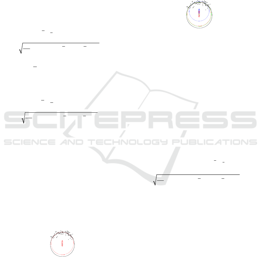
samples are taken. The dashed bar in Figure 3 show

that the true center is not anywhere within the error

ellipsoid of the estimate. This is due solely to the

bias in the estimator. This is a good example of why

the GDKE has not been adopted as much as the

others.

NEW CLOSED FORM SOLUTIONS FOR SKELETAL EXTRACTION FROM MOTION CAPTURE

251

Figure 3: GDKE error ellipse.

5 GENERALIZED

DELOGNE-KASA EXPOSITION

The Generalized Delogne-Kása (GDK) estimator

(Strandlie, 2000) is the starting basis for our new

formulae. This estimator is a general solution for

finding the best-fit hypersphere from measurements

on the surface. However until now the estimator has

limited uses as the estimator is biased and can

produce significantly different answers from the

solution. The GDK estimator provides a good

estimate if the data is evenly distributed over the

entire surface of the hypersphere. The estimate falls

farther away as the data gets clumped to one side.

The GDK estimator is derived from surface

measurements x

and their deviation from a fixed

distance from the center. The deviation for N

measurements is written as

GDK

()

N −1

−

()

−

()

−

()

i=1

∑

(1)

The minimization of this (Knight, 2008)

produces estimations for the center and the radius

c =

x +

−1

(2)

−

()

−

()

i=1

∑

(3)

where the intermediate quantities include the

arithmetic vector mean

x =

i=1

∑

(4)

and the variance-covariance matrix

C =

N−1

− x

()

− x

()

i=1

∑

(5)

and the third central vector moment

S =

N−1

− x

()

− x

()

− x

()

i=1

∑

(6)

This estimation of the hypersphere is very fast

due to the Cholesky inverse. The floating point

operations for a D-dimensional hypersphere can be

counted as

FLOPs = ND

+ 6 D − 1

(

)

DD+ 1

()

D + 8

()

+ 1

(7)

which, for the sphere, is

LOPs

(8)

This estimator is about as fast as you can get for

this problem but it has one fatal flaw. The estimator

has been shown to be biased providing an answer

that is offset even under fairly normal conditions.

The bias is proportional to the variance of the data

(Zelniker, 2004) but analysis here shows the

multiplication factor can outweigh an accurate

measurement. The bias comes from the fact that one

of the variables in the center equation is biased. We

consider a measurement system that has a consistent

error for each measurement on the surface of the

sphere. The measurement is expected to be on the

surface but varies from it by the multi-dimensional

Gaussian distribution thus

= Gaussian

, Σ

(

)

(9)

The covariance matrix is then expected to be

E C

(

)

(10)

N−1

−

()

−

()

∑

(11)

E S

(

)

(12)

N−1

−

()

−

()

−

()

∑

(13)

()

= c

+Σ

()

−1

− C

−1

(

)

(14)

6 UNBIASED GDK

Unbiased GDK provides a quick method to draw a

skeleton from motion capture data. The main

contribution to the state of the art is that the

estimator explained below is asymptotically

unbiased. Asymptotically unbiased is defined as an

inversely proportional relationship with the sample

count:

(

)

(

)

where q

is the parameter

that the estimator is trying to estimate. This basically

says that the estimator is expected to get closer to

the true answer if more samples are taken. It is

shown in (Knight, 2008) that the GDKE estimators

for center and radius do not satisfy this requirement.

GRAPP 2009 - International Conference on Computer Graphics Theory and Applications

252

Our algorithm uses a simple substitution that turns

the GDKE into one with a diminishing bias. It

involves the use of an a-priori estimate of the

measurement error in the samples. This is very

reasonable since most systems of measurement have

some kind of estimate to the measurement error.

Since the sample covariance matrix C is the only

biased term in the equation for the GDKE center,

this is what will be altered.

′

C = C−

(15)

E C −

()

= C

+Σ−

(16)

= x +

C −

()

−1

(17)

N −1

Tr C −

()

+ x −

()

x −

()

(18)

()

− c

()

− c

()

i=1

∑

− r

(19)

This leads to fastest, asymptotically unbiased

estimator of a hypersphere in (Knight, 2008) as

′

c =

x +

C−

()

−1

(20)

′

r =

N−1

Tr C−

()

+ x −

′

()

x −

′

()

(21)

A typical use of these new estimators can be

displayed using Mathematica, with exactly the same

data as used for displayed for the GDKE. The true

center is within the error ellipsoid (Figure 4). This

data contains 100 points generated with a diagonal

measurement covariance with all diagonals equal to

0.05

. The Leontief condition (

) is satisfied with

the spectral radius in question equal to 0.557238.

These equations show that there still is a bias, but it

is asymptotically unbiased. We implemented (results

in Figure 4). A Monte-Carlo run that explicitly

shows the 1/√N dependency. The error in the

estimate is compared with how many points were

analyzed for a particular joint in given motion

capture data.

Figure 4: UGDK error ellipse.

An example analysis using MLE, UGDK and

GDKE is presented in Figure 5. The figure clearly

shows the improvement over the GDKE with same

FLOP count for UGDK as GDKE. The figure shows

the bias is removed using the UGDK and results

produced by UGDK are close to MLE. The FLOP

counts for UGDK remains same as GDK (Knight

2008). Our analysis in (Knight 2008) also shows that

there is a case when all methods have troubles in

estimating the joint location – this is the case when

measurement error is actually bigger than the item

being measured. This situation is a bit impractical,

as no one wants such a system of measurement.

Figure 5: Comparison of methods.

7 NEW SOLUTION: MULTIPLE

RADII SOLUTION

For multiple markers going around the same center

of rotation, another formula can be achieved by the

same analysis of least squares. This technique is

good to use when more than one marker is available.

It has the ability to average out errors when one

marker is too close to the rotation point or has other

systematic problems. Excluding the derivation, we

have the following equations for center and radius

estimates where M is the number of markers and

subscript p indicates values that utilize the single

marker’s positions:

= C

−

()

p=1

∑

⎛

⎝

⎜

⎞

⎠

⎟

−1

−

()

p=1

∑

(22)

N −1

Tr C

−

(

)

+ x

−

()

−

()

(23)

Symbols and conventions are given in Section 2.

The matrix that is to be inversed here is still a

positive-definite matrix since positive-definite

matrices added together still produce a positive-

definite matrix. This allows for the speedier

Cholesky decomposition and the singular values can

be excluded. An example of the MGDK method is

presented in Figure 6. This example shows what

happens when the individual circles are compared to

that when combined in the MGDK. The outer circle

solution is drawn in red; the inner circle solution is

drawn in blue, and the MGDK solution is drawn in

green. The example shows a dramatic improvement

over both of the individual circle calculations. FLOP

count analysis is in (Knight, 2008).

NEW CLOSED FORM SOLUTIONS FOR SKELETAL EXTRACTION FROM MOTION CAPTURE

253

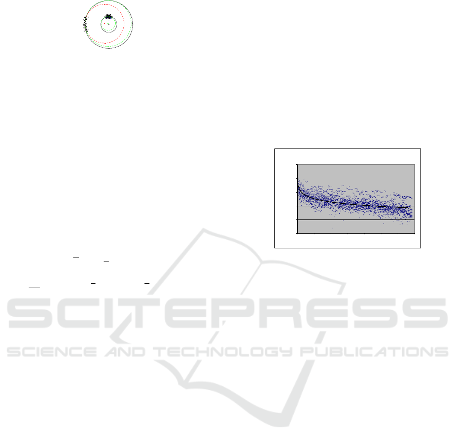
Figure 6: Comparison of methods.

8 NEW SOLUTION: IGDK

A more refined answer can be achieved when using

a incremental improvement GDK (IGDK) formula.

The idea here is a group of samples are collected and

an answer is retrieved from the GDKE or UGDK

formulae. Excluding the derivation, we have the

following equations. Equations for S and C for

(n+1)th sample are defined in (Knight, 2008) and are

calculated using recurrence relationship. Below are

the final equations for the center and radius. The

advantage is that no new matrix inverse is needed

and the storage requirements are of constant order.

n+1

= x

n+1

−1

n+1

(24)

n+1

Tr C

n+1

()

+ x

n+1

−

n+1

()

n+1

−

n+1

()

(25)

When compared to the FLOPs for the GDKE

method, this incremental approach is about four

times slower. This makes the incremental approach a

last resort when a few extra points need to be added

to a previously calculated center and radius. This

new estimator has the distinct advantage of constant

memory requirements no matter how many points

are analyzed.

9 EXPERIMENTS

9.1 Case Study – CMU Data

The CMU Graphics Lab produced a one minute long

motion capture data-set of a salsa dance in 60-08.

The data file contains 3421 time slices for 41

markers on two figures. This case study will

concentrate on analyzing the performance of the

UGDK in determining the rotation points in the

female subject. Four data sets were created by

removing random samples from the CMU data sets.

400 rotation points were collected. The calculated

constants are the relative rotation points as

referenced in each segment’s parent’s coordinate

system. The 400 calculations were averaged and the

standard deviations were calculated as well. Details

results are analyzed in (Knight, 2008) Most of the

standard deviations are less than one centimeter, but

there are some significant outliers like the right

ankle. Further analysis of the calculated points for

the ankles and elbows shows that the four runs

produced two answers due to different orientations

of the parent’s reference frame. As can be readily

seen from the above graph, a statistically significant

amount of calculations are within one centimeter of

accuracy when analyzing more than about 200

samples. The accuracy gets better on average with a

power law close to 1/√N (Figure 7). Skeletal

animation of our results is provided in mpeg files.

Deviation From Mean Rotation Point

y = 0.5117x

-0.8125

0.00001

0.0001

0.001

0.01

0.1

0 500 1000 1500 2000 2500 3000 3500

Number of Samples

Figure 7: Inverse Power Law.

9.2 Case Study of Eric Camper’s

ACCAD Data

The motion capture data in the ericcamper.c3d

(Motion was analyzed to produce a skeleton. The

subject did various martial arts maneuvers that

moved every joint involved in drawing. One time

frame is presented in the following figure. We show

a frame of animation in Figure 1 which shows what

appears to be a natural pose for all joints during a

karate exercise.

10 RESULTS

A Monte-Carlo experiment was set up to determine

the speed of the various sphere-fit algorithms. Up to

a million samples were chosen on a sphere with

varying measurement error, confinement angle,

sphere-center and sphere-radius. The measurement

error varied from 1x10

-11

to 1x10

. The confinement

angle varied from 0 to 180°. The sphere center

varied as much as 2 around the origin. The radius

varied 0 to 37. The linear algebra algorithms were

all implemented from well-accepted

implementations presented in Numerical Recipes in

C (Press, 1992) The code was compiled optimized

for a PowerPC G4 processor and run on a 1GHz

Apple PowerBook 12”.

GRAPP 2009 - International Conference on Computer Graphics Theory and Applications

254

As discussed in (Knight, 2008), the GDKE, and

therefore UGDK, is always faster with FLOP count

as 26 N. The GDKE/UGDK is 2.17 times faster than

IGDK on average. Based on FLOP counts as

explained in (Knight, 2008) in detail, the

GDKE/UGDK is 11.05 times faster than the LLS

method and about 80 times faster than the MLE

when the measurement error is less than one.

10.1 Summary of Important Results

Three new closed-form methods have been

presented to find rotation points of a skeleton from

motion capture data. A generic skeleton can be

directly extracted from noisy data with no previous

knowledge of skeleton measurements. The new

methods are ten times faster than the next fastest and

a hundred times faster than the most widely accepted

method. Two phases are used to produce an accurate

skeleton of the captured data. The first phase, fitting

the skeleton, is robust even with noisy motion

capture data. As explained earlier, the formulae use

an asymptotically unbiased version of the

Generalized Delogne-Kása (GDKE) Hyperspherical

Estimation (i.e UGDK). The second estimator takes

advantage of multiple markers located at different

distances from the rotation point (MGDK) thereby

increasing accuracy. The third estimator

incrementally improves an answer and has

advantages of constant memory requirements

suitable for firmware applications (IGDK). The

UGDK produces the answer faster than any previous

algorithm and with the same efficiency with respect

to the Cramér-Rao Lower Bound for fitting spheres

and circles. The UGDK method significantly

reduces the amount of work needed for calculating

rotation points by only requiring 26N flops for each

joint. The next fastest method, Linear Least-Squares

requires 236N flops. In-depth statistical analysis

shows the UGDK method converges to the actual

rotation point with an error of O(σ/√N) improving

on the GDKE’s biased answer of O(σ). The second

phase is a real-time algorithm to draw the skeleton at

each time frame with as little as one point on a

segment. This speedy method, on the order of the

number of segments, aids the realism of motion data

animation by allowing for the subtle nuances of each

time frame to be displayed. Flexibility of motion is

displayed in detail as the figure follows the captured

motion more closely. With the reduced time

complexity, multiple figures, even crowds can be

animated. In addition, calculations can be reused for

the same actor and marker-set allowing different

data sets to be blended.

11 CONCLUSIONS

In our effort to try to speed up skeleton extraction

from motion capture date we discovered a new

asymptotically unbiased GDK (UGDK) formulation

which fills the vital low-level hole and makes GDK

formulation practical. This paper presents the fastest

known general method for calculating the rotation

points and can be as much as ten times faster than

the next fastest method available as explained in

(Knight, 2009) The UGDK method has further

impact in a vast collection of fields as diverse as

character recognition to nuclear physics where an

algorithm is needed for the speedy recovery of the

center of a circle or sphere. The UGDK is expected

to play a vital role in the process of determining a

skeleton from motion capture data. The MGDK adds

robustness to the equations allowing to use every bit

of available data. The IGDK further has the

application of being an ideal algorithm to burn into a

silicon chip whose memory requirements are

constrained.

The UGDK estimators are an improvement on

existing science but they are strictly dependent on a-

priori knowledge of the measurement error. It has

been shown that the measurement error trace can

itself be estimated but not the whole measurement

covariance matrix. An estimator for the whole

matrix would be most ideal but was not found in the

course of this study and should be a topic of future

research. The main contributions are the new

unbiased center formulae; the full statistical analysis

of this new formula; and the analysis of when the

best measurement conditions are to initiate the

formula. The research further establishes the

application of these new formulae to motion capture

to produce a real-time method of drawing skeletons

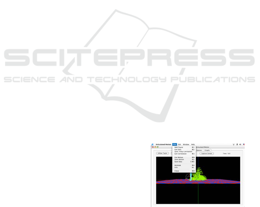
of arbitrary articulated figures. is advisable to keep

all the given values.

Figure 8: A sample of File menu interface.

NEW CLOSED FORM SOLUTIONS FOR SKELETAL EXTRACTION FROM MOTION CAPTURE

255

ACKNOWLEDGEMENTS

We wish to thank all the reviewers of the paper,

especially numbers 3 and 4, for their insightful

comments.

REFERENCES

Aguiar, D., Theobalt, C., Seidal,H., Automatic learning of

articulated Skeletons from 3D marker Trajectories, in

International Symposium, ISVC 2006, part I, Springer-

Veralag, Lecture Notes in Computer Science, vol.

4291, pp. 485-494 (2006).

O’Brien, J. F., Bodenheimer Jr R. E. ., Brostow G. J., and

Hodgins J. K..

Automatic Joint Parameter Estimation

from Magnetic Motion Capture Data

, pages 53–60,

Montreal, Quebec, Canada, May 15-17 2000. Graphics

Interface.

Burr, M., Cheng, A., Coleman, R., and Souvaine, D.,

Transformations and Algorithms for Least Sum of

Squares Hypersphere Fitting.

Canadian

Conference on Computational Geometry,

2004, pp

104-107.

Camper, E., Motion Capture Data accaccad.osu.edu/

research/mocap/mocap_research.html

Corral, C., Lindquist, C., On implementing Kása’s circle

fit procedure.

IEEE Transactions on Instrumentation

and Measurement

, 47(3):789–795, June 1998.

Delogne, P.,Computer Optimization of Deschamps

Method and Error Cancellation in Reflectometry. In

Proceedings of the IMEKO Symposium on Microwave

Measurements

, Budapest, Hungary, May 1972, pp.

117-129.

Gander, W., Golub, G., Strebel, R., Least-Squares Fitting

of Circles and Ellipses.

BIT Numerical Mathematics

34, Springer 1994, pp 558-578.

Herda, L., Fua, P., Plankers, R., Boulic, R., D. Thalmann,

D., Skeleton-based motion capture for robust

reconstruction of Human Motion, Computer

Animation (book), Philadelphia, PA, pp.77-May

(2000).

Kása, I., A circle fitting procedure and its error analysis.

IEEE Transactions on Instrumentation and

Measurement

, 25:8–14, March 1976.

Kirk, A. G., O’Brien, J., Forsyth, D.A. Skeletal parameter

estimation from optical motion capture data. In

IEEE

Conf. on Computer Vision and Pattern Recognition

(CVPR). IEEE, 2005.

Knight, J., Semwal, S., Fast Skeleton estimation from

motion captured using Genralized Delogne-Kasa

method, In

International Conference in Central

Europe on Computer Graphics, Visualization and

Computer Vision, Plzen, WSCG Conference

Proceedings, pp. 225-232, ISBN 978-80-86943-98-5,

Feb 2007.

Knight, J., Rotation Points from Motion Capture Data

using a closed form solution,

PhD thesis, University of

Colorado at Colorado Springs, Advisor Professor

Semwal, SK., pp. 1-152 (2008).

Lukács, G., Marshall, A., Martin, R., Geometric Least-

Squares Fitting of Spheres, Cylinders, Cones, and Tori

RECCAD Deliverable Documents 2 and 3 Copernicus

Project No. 1068

Reports on basic geometry and

geometric model creation, etc. Edited by Dr. R. R.

Martin and Dr. T. Varady Report GML 1997/5,

Computer and Automation Institute, Hungarian

Academy of Sciences, Budapest, 1997.

Pratt, V., Direct least-squares fitting of algebraic surfaces.

Computer Graphics, 21(4):145–152, July 1987.

Press, W., Teukolsky, T., Vetterling, W., Flannery, B.,

Numerical Recipes in C: The Art of Scientific

Computing. 2nd.ed., Cambridge University Press:

1992.

Robinson, S.Fitting Spheres by the Method of Least

Squares,

In Communications of the ACM, Volume 4,

No. 11; November 1967, p. 491.

Shakarji, C., Least-Squares Fitting Algorithms of the

NIST Algorithm Testing System,

J. of Research of the

National Institute of Standards and Technology

: 103,

No. 6 (1998): 633.

Strandlie, A., Wroldsen, J., Frühwirth, R., and

Lillekjendlie, B.,Track Fitting on the Riemann Sphere.

International Conference on Computing in High

Energy and Nuclear Physics

, Padova, Italy; February,

2000.

Thomas S., Chan, Y., Cramer-Rao Lower Bounds for

Estimation of a Circular Arc Center and Its’ Radius.

CVGIP: Graphics Model and Image Processing, Vol.

57, No. 6, pages 527-532, 1995.

Witte, L.. Least Squares Fitting of a Great Circle Through

Points on a Sphere.

Communications of the ACM,

Volume 3, No. 11, November 1960, pp. 611-613.

Zelniker E., Clarkson, I., A Statistical Analysis Least-

Squares Circle-Centre Estimation. In

IEEE

International Symposium on Signal Processing and

Information Technology

, December 2003, Darmstadt,

Germany, pp 114-117.

Zelniker, E., Clarkson, I., A Generalisation of the

Delogne-Kása Method for Fitting Hyperspheres.

Thirty-Eighth Asiomar Conference on Signals,

Systems and Computers.

Pacific Grove, California,

November 2004.

GRAPP 2009 - International Conference on Computer Graphics Theory and Applications

256