UATION DISCOVERY FOR MACROECONOMIC MODELLING

Dimitar Kazakov

Department of Computer Science, The University of York, YO10 5DD, York, U.K.

Tsvetomira Tsenova

European Central Bank, Frankfurt am Mein, Germany

Bulgarian National Bank, Soﬁa, Bulgaria

Keywords:

Machine learning, Equation discovery, LAGRAMGE, Macroeconomic modelling, Inﬂation.

Abstract:

This article describes a machine learning based approach applied to acquiring empirical forecasting models.

The approach makes use of the LAGRAMGE equation discovery tool to deﬁne a potentially very wide range of

equations to be considered for the model. Importantly, the equations can vary in the number of terms and types

of functors linking the variables. The parameters of each competing equation are automatically ﬁtted to allow

the tool to compare the models. The analysts using the tool can exercise their judgement twice, once when

deﬁning the equation syntax, restricting in such a way the search to a space known to contain several types

of models that are based on theoretical arguments. In addition, one can use the same theoretical arguments to

choose among the list of best ﬁtting models, as these can be structurally very different while providing similar

ﬁts on the data. Here we describe experiments with macroeconomic data from the Euro area for the period

1971–2007 in which the parameters of hundreds of thousands of structurally different equations are ﬁtted and

the equations compared to produce the best models for the individual cases considered. The results show the

approach is able to produce complex non-linear models with several equations showing high ﬁdelity.

1 INTRODUCTION

Understanding the nature of the inﬂation process is a

central issue in macroeconomics.

The private agents,

businesses and households alike, are interested in its

forecasting, as expectations on inﬂation, and other

key macro-variables, affect the way in which they

make their investment and saving decisions and nego-

tiate labour contracts. Policy makers, especially those

in charge of monetary policy, are interested in both

forecasting and control of inﬂation.

The general characteristics of the inﬂation pro-

cess, as well as the structure of the economy are

evolving through time. After the 1980s, inﬂation lev-

els have declined in the industrialised countries, coin-

ciding with low volatility of both inﬂation and output,

less pronounced and shorter business cycles (Stock

and Watson, 2003). Many have speculated on the

potential sources of this phenomenon, also known as

All

opinions are those of the authors and do not imply

agreement or endorsement by the European Central Bank or

the University of York.

the Great Moderation — successful monetary policy,

globalisation, ﬁnancial markets developments (over-

coming of ﬁnancial costs and borrowing constraints

for both residential and business investment), or good

fortune. With the sudden collapse of the ﬁnancial

markets in the last few weeks, it is possible that this

period of stability may be followed by a transitional

period while the system switches to a new regime.

This is likely to further fuel the discussion on the un-

derstanding of the underlying processes and the way

in which they are modelled. We believe that this dis-

cussion should be informed by both theoretical insight

and analysis of the empirical data.

With this work, we want to attract the attention

to a machine learning approach, combining these two

aspects through the search for empirical models in

which the chosen functional dependencies between

the system variables are economically sound, but the

actual functional form of these dependencies is se-

lected from a much wider than usual spectrum of

options. We use a dataset of macroeconomic ob-

servations from the Euro area and supply the LA-

318

Kazakov D. and Tsenova T. (2009).

EQUATION DISCOVERY FOR MACROECONOMIC MODELLING.

In Proceedings of the International Conference on Agents and Artiﬁcial Intelligence, pages 318-323

DOI: 10.5220/0001802403180323

 SciTePress

GRAMGE equation discovery tool used here with a

range of grammars describing the possible syntax

(functional terms, dependencies between variables,

maximum complexity) of each equation. The recur-

sive empirical models produced as a result are tested

on their ability to (1) predict the next state of the sys-

tem from past observations for the data used to learn

the model (i.e., using training data to measure the “in-

sample” error), (2) predict the next state from past ob-

servations for data not used in the training (using the

test data to measure “out-of-sample” error), and, ﬁ-

nally, (3) forecast the future of the system (parameter

in question) starting from the last observation used in

training, and recursively using the model’s own pre-

dictions to look another step ahead in time. The re-

sults suggest that the empirical approach is able to re-

produce the results of other approaches, when simi-

larly constrained, and go further to produce complex

nonlinear models able to forecast inﬂation over con-

siderable periods of time.

2 BACKGROUND

2.1 Empirical Modelling of the Inﬂation

Process

In addition to the observed decline in inﬂation volatil-

ity in recent years, the inﬂation had grown increas-

ingly disconnected from other macro variables. The

inﬂation process can be modelled as a function of its

own history, in which the possibility of a time trend

is also taken into account. Linear estimations of that

kind are known to produce forecasts that are hard to

outperform in terms of out of sample accuracy. There-

fore, the ﬁrst model to consider here is a univariate

autoregressive model of the general form:

= f (π

t−1

, π

t−2

. . . π

t−k

, t) (1)

where π

is the inﬂation rate and t is time.

This type of modelling does not provide, however,

a satisfactory understanding on the co-movement and

dependence between the nominal and the real side of

the economy (i.e., inﬂation and output) and how these

are inﬂuenced by monetary policy (interest rates).

Economic theory suggests that inﬂation is linked to

output y (Eq. 3), more speciﬁcally, it rises when

output increases over a certain level, a relationship

known as the Phillips curve. Similarly, output is cor-

related with the interest rate r (Eq. 2), and is expected

to rise when interest rates are lowered, a relationship

known as the IS (Investment and Saving) curve (Blan-

chard, 2000). Monetary policy is supposed to react to

inﬂation, as well as the state of the economy mea-

sured through its output, which is a relationship re-

ﬂected in Eq. 4. Here the most common approach is

to model these three equations as linear functions. It is

suggested though that due to the constantly evolving

structure of the economy, a linear speciﬁcation could

fail in capturing those relationships and might under-

estimate their value for forecasting.

= f (y

t−1

, y

t−2

, ...r

, r

t−1

, ...t) (2)

= f (π

t−1

, π

t−2

, ...y

, y

t−1

, ...t) (3)

= f (π

, π

t−1

, ...y

, y

t−1

, ..., t) (4)

2.2 Machine Learning, Equation

Discovery and LAGRAMGE

Machine Learning (ML) aims at describing the prop-

erties of a set of observations from a given source,

and/or making predictions about the nature of future

observations from the same source. Both goals are

achieved by changing the representation of available

data as expressed in its original form (or object lan-

guage) into another representation (using another for-

malism, known as hypothesis language). The new

representation copies closely the information encoded

in the original data, but is usually more general, and

allows statements to be made about yet unseen cases.

ML can be seen as the search for a mapping from a set

of inputs to an output; this mapping is often a func-

tion. In the context of searching for macroeconomic

models, this means functional relationships between

the observed variables can be determined.

No ML algorithm can make predictions unless it

employs a bias (Mitchell, 1997). In general, the bias

will restrict the range of possible functions (models,

hypotheses) that can be described by the hypothe-

sis language. For instance, the set of data points

{(0, 0), (π, 0), (2π, 0)} can be modelled by the func-

tions y = 0, y = cos x or y = x(x − π)(x − 2π), de-

pending on the bias, which may restrict the hypothesis

to a linear, trigonometric or polynomial function.

Such a bias is also called language bias to distin-

guish it from the preference bias, allowing a choice

between alternative models with equal coverage of

the available data. Here some simple, but general

principles (heuristics) are often employed. For in-

stance, Occam’s razor (Mitchell, 1997) favours the

simplest hypothesis language, while the Minimal De-

scription Length (MDL) bias (Rissanen, 1978) sug-

gests a trade-off between the complexity of the hy-

pothesis language and that of the resulting represen-

tation of the data.

The area of ML focusing on the search for quanti-

tative laws, expressed as equations, is known as equa-

EQUATION DISCOVERY FOR MACROECONOMIC MODELLING

319

Table 1: Sample data.

Quarter/Year π y r

1971Q1 5.25 4.22 0.68

1971Q2 5.83 3.56 -0.16

1971Q3 6.09 3.92 -0.14

1971Q4 6.36 3.50 -0.21

2007Q1 1.87 3.07 1.93

tion discovery. The system LAGRAMGE (Todorovski

and D

zeroski, 1997) is one example of this approach.

When an initial draft of the equation is provided, the

process is known as equation revision (Todorovski

and D

zeroski, 2001). In this case, initial input is re-

quired from experts, but the changes carried out by the

learner can be non-trivial, and result in large improve-

ments (Todorovski et al., 2003). A unique feature of

LAGRAMGE is its use of a user-deﬁned context-free

grammar to deﬁne a potentially different language

bias for each modelling task. Here the range of pos-

sible equations is deﬁned at a symbolic level, and the

actual parameters (constants) of the equations consid-

ered in the search are ﬁtted automatically in the pro-

cess. A set of simple constraints, such as the maxi-

mum depth of the equation parse tree, are employed

to prune the search and make it feasible. Even with

such restrictions, the search is often conducted over a

potential range of hundreds of thousands of different

equations. LAGRAMGE can also be set to use a form

of an MDL preference bias to penalise for additional

complexity of the equations found.

2.3 The Euroarea Dataset

The dataset used consists of quarterly data of the an-

nual rates of inﬂation π, output growth y, and the

nominal interest r for the Euro area in the period

1971Q1–2007Q1 (see Table 1). The dataset was di-

vided into data used for model estimation (i.e., train-

ing sample/dataset, comprising all readings in the pe-

riod 1971Q1–2005Q1), and a test dataset 2005Q2–

2007Q1, which was used to evaluate the models on

previously unseen data (“out-of-sample evaluation”).

Wherever the real interest rates were needed, they

were assumed to be equal to the nominal interest rates

minus the realised (i.e., actual) inﬂation one period

ahead, the latter being used as a proxy for the ex-

pected inﬂation rate.

2.4 Experimental Design

All models are obtained by designating an output

variable in the dataset, and specifying the range of

other variables that are to be considered as indepen-

dent variables in the equation. This is repeated un-

til equations for all output variables in the model are

obtained. We also have to specify the operators and

functors that may appear in each equation. In all

cases, the equations can be expressed as sums of some

the following types of terms:

• A constant: c.

• A product of a constant and a variable: c

• A product of a constant and two variables:

• A product of a constant, a variable, and a sin func-

tion of a linear function of the same or other vari-

able: c

.sin(c

+ c

• A product of a constant, and two sin func-

tions with arguments as above: c

.sin(c

).sin(c

+ c

The above range makes possible to describe a

range of linear and non-linear equations that will be

considered by the learner.

3 RESULTS AND EVALUATION

Firstly, we estimate a baseline linear autoregressive

model – inﬂation as a function of its previous two

values – using standard tools (Matlab). The resulting

equation is:

= 0.04 + 1.49π

t−1

− 0.50π

t−2

+ ε

ε ∼ iid N

0, σ

(5)

where ε is the model’s error. Using LAGRAMGE

to perform the same task produces the following equa-

tion:

= 0.06 + 1.38π

t−1

− 0.40π

t−2

+ ε

(6)

The evaluation of the accuracy of the models is

performed according to the root mean squared error

(RMSE), and mean absolute error (MAD).

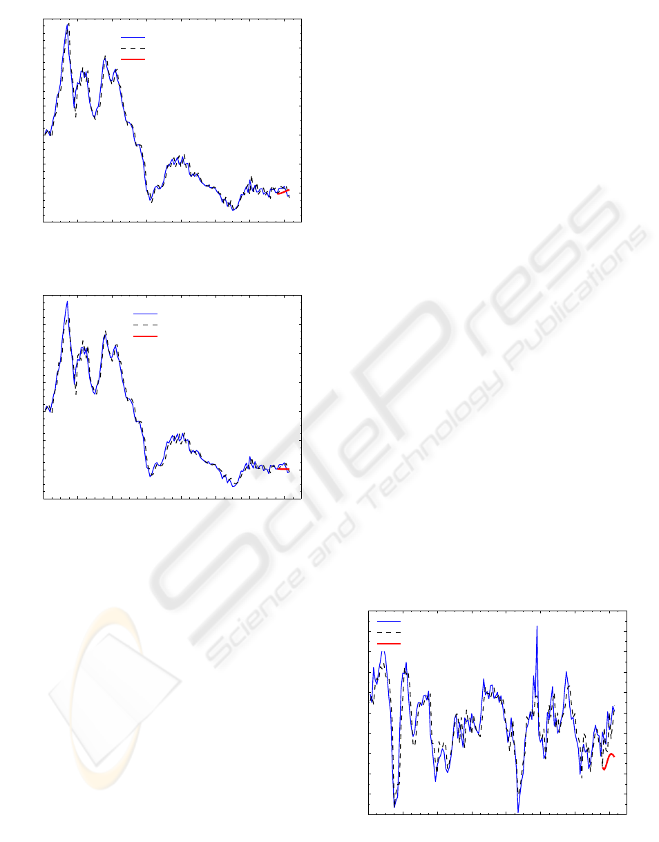
The baseline and the LAGRAMGE model have al-

most identical accuracy - with the out of sample ac-

curacy greater than the in-sample accuracy. Figure

1 shows the in-sample ﬁt (up to 2005Q1) and out of

sample (from 2005Q2 onwards) forecasts.

Non-linear models relax the language bias and al-

low for potentially more complex and accurate mod-

els (Clements et al., 2004). The full capabilities of

LAGRAMGE are used when looking for non-linear

speciﬁcations. The best equation has an inﬁnitesimal

time trend which is unlikely to be signiﬁcant. (It also

produces inferior out of sample forecasts). Therefore

we skip to the second-best equation, reported below:

ICAART 2009 - International Conference on Agents and Artificial Intelligence

320

75Q4 80Q4 85Q4 90Q4 95Q4 00Q4 05Q4

Actual

One step ahead estimation and forecast

Recursive forecast

Figure 1: Inﬂation π: actual rate (in %) vs linear model one-

step-ahead forecast and recursive out-of-sample forecast.

75Q4 80Q4 85Q4 90Q4 95Q4 00Q4 05Q4

Actual

One step ahead estimation/forecast

Recursive − out of sample

Figure 2: Inﬂation π: actual rate (in %) vs non-linear model

one-step-ahead forecast and recursive out-of-sample fore-

cast.

= −0.51 + 0.89π

t−1

3.26sin(−0.19π

t−2

+ 1.99) −

2.51sin(−0.28π

t−1

− 4.12) (7)

The accuracy of this non-linear autoregressive

model is shown in Fig. 2.

The next class of models learned assumes that

forecasts are based on a system of equations, as de-

scribed in Eq. 2–4. The best equation, in terms of

in-sample ﬁt, on the real interest rate provides us with

the following equation:

= (8)

6.98 + 0.05y

t−2

8.88sin(0.09r

t−1

− 32.21) sin(0.05π

t−1

+ 14.18) +

23.14sin(0.01π

t−2

+ 0.01) sin(0.045t −1.78) + ε

For the output we choose the third best equation,

since the previous two have an insigniﬁcant trend and

are rejected on theoretical grounds:

= (9)

1.60 + 0.07y

t−2

8.84sin(0.11r

t−2

+ 1.20) sin(0.58y

t−1

+ 0.84) +

10.66sin(0.56y

t−1

− 2.02) sin(0.11y

t−2

+ 0.88)

The inﬂation equation is LAGRAMGE’s second

best and the ﬁrst that satisﬁes the human expert:

= (10)

0.11 + 0.96π

t−1

6.65sin(0.60y

t−1

− 1.02) sin(0.02π

t−1

− 0.04) −

0.62sin(−0.28π

t−1

+ 0.71) sin(0.21t −1.09)

Note that the graphs in Fig.1–5 up to 2005Q1 rep-

resent the in-sample ﬁt, that is, how well the model

anticipates a data point that has been used in extract-

ing the model. Past the 2005Q1 point, the one-step

ahead projections are true out-of-sample predictions

– LAGRAMGE had no knowledge of those data points

while learning the model; when the model is used,

each of the actual data readings was fed to the model

to predict its value in the next time interval. Out-of-

sample prediction was also carried out in a recursive

manner, starting from the last known data point, mak-

ing a one step ahead prediction, then using it as a start-

ing point to make a forecast for the next time interval.

Of course, the recursive forecast is the hardest of all,

as its errors are gradually accumulated.

The accuracy of Eq. 5–10 are evaluated in Table 2.

It is reassuring that the out-of-sample accuracy of all

equations on inﬂation (Eq.5–7, 10) is greater than

the in-sample accuracy, as it suggests that the mod-

els have genuinely captured some of the properties of

the system, and have predictive power, rather than just

being an overﬁtted model of the training data.

75Q4 80Q4 85Q4 90Q4 95Q4 00Q4 05Q4

−2

−1

Actual

One step ahead estimation/forecast

Recursive − out of sample

Figure 3: Output y: actual rate versus non-linear multi-

variate model one-step-ahead forecast and recursive out-of-

sample forecast.

EQUATION DISCOVERY FOR MACROECONOMIC MODELLING

321

75Q4 80Q4 85Q4 90Q4 95Q4 00Q4 05Q4

−4

−2

Actual

One step ahead estimation/forecast

Recursive − out of sample

Figure 4: Real interest r: actual rate versus non-linear mul-

tivariate model one-step-ahead forecast and recursive out-

of-sample forecast.

4 DISCUSSION

The univariate non-linear model of inﬂation (Eq. 7 is

the best of all; it outperforms the baseline on all mea-

sures, and its superiority is particularly evident in the

most important aspect, the recursive out-of-sample

prediction, where its error is almost half of that of the

baseline model. Some of the most recent advances in

macroeconomic modelling have

75Q4 80Q4 85Q4 90Q4 95Q4 00Q4 05Q4

Actual

One step ahead estimation/forecast

Recursive − out of sample

Figure 5: Inﬂation π: actual rate versus non-linear multi-

variate model one-step-ahead forecast and recursive out-of-

sample forecast.

been based on the iterative re-estimation of the

model parameters with each new observation.

Not so here – all our models hold their ground for

a period spanning 34 (resp. 36) years, without the

need for adjustment. This increases the likelihood

that they may offer some theoretical insight rather

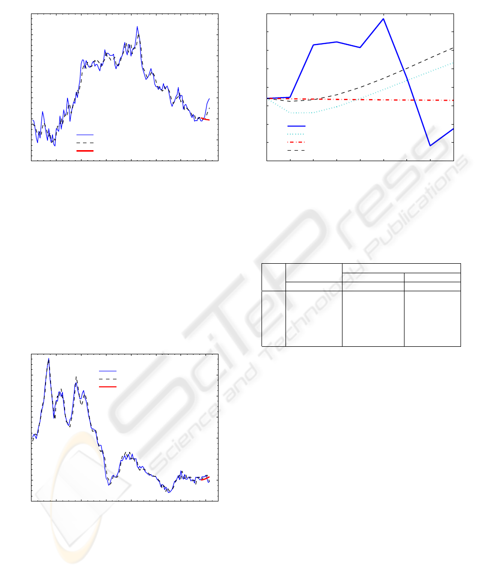
05Q1 05Q2 05Q3 05Q4 06Q1 06Q2 06Q3 06Q4 07Q1

1.7

1.8

1.9

2.1

2.2

2.3

2.4

2.5

Actual

Linear univariate model

Non−linear univariate model

Non−linear multivariate model

Figure 6: Inﬂation π: a close-up comparison of recursive

out-of-sample forecasts.

than just being a numerical tool minimising error. The

Table 2: RMSE - root mean squared error; MAD - mean

absolute deviation.

Eqn In-sample Out-of-sample

One step ahead Recursive

RMSE MAD RMSE MAD RMSE MAD

5 0.49 0.36 0.22 0.19 0.46 0.41

6 0.49 0.36 0.22 0.19 0.46 0.41

7 0.45 0.34 0.20 0.15 0.26 0.23

8 0.56 0.45 0.64 0.52 1.15 0.87

9 0.83 0.64 1.13 0.95 1.82 1.75

10 0.38 0.30 0.23 0.16 0.31 0.26

more complex, 3-equation model performed less well,

which may be due to the fact that it combined three

different forecasts, each with its own systemic er-

ror; however, this inﬂation forecast still outperformed

the baseline. There are other interesting aspects of

this model—for instance, when used in a recursive

forecast mode, it can spontaneously go in and out

of an auto-oscillation regime. This is signiﬁcant, as

it demonstrates the potential ability of the learner to

produce models describing different regimes (modes)

of the system within the same equations. There is a

lot more work to be done, with learning differential

equations, splitting the training data at points of ma-

jor structural changes in the EU, and modifying the

language bias being only some of the options.

REFERENCES

Blanchard, O. (2000). Macroeconomics. Prentice Hall, sec-

ond edition.

Clements, M. P., Franses, P. H., and Swanson, N. R. (2004).

Forecasting economic and ﬁnancial time-series with

ICAART 2009 - International Conference on Agents and Artificial Intelligence

322

non-linear models. International Journal of Forecast-

ing, 20:169–183.

Mitchell, T. (1997). Machine Learning. McGraw-Hill.

Rissanen, J. (1978). Modeling by shortest data description.

Automatica, 14:465+.

Stock, J. and Watson, M. (2003). Has the business cycle

changed? Evidence and explanations. In FRB Kansas

City Symposium.

Todorovski, L. and D

zeroski, S. (1997). Declarative bias

in equation discovery. In Proc. of 14

International

Conference on Machine Learning, pages 376–384.

Todorovski, L. and D

zeroski, S. (2001). Theory revision

in equation discovery. In Proc. of the 4

Interna-

tional Conference on Discovery Science, volume 2226

of LNCS, pages 389+. Morgan Kaufmann.

Todorovski, L., D

zeroski, S., Langley, P., and Potter, C.

(2003). Using equation discovery to revise an Earth

ecosystem model of carbon net production. Ecologi-

cal Modelling, 170:141–154.

EQUATION DISCOVERY FOR MACROECONOMIC MODELLING

323